Real-World RL
Core idea. Real-World RL targets critic and policy learning from streaming interactions with the real system. The goal is to learn task-level value and decision structure—not merely to fit the latest closed-loop trajectory. The current BOCO evidence is a critic-learning and primal-control precursor within this broader Theme.
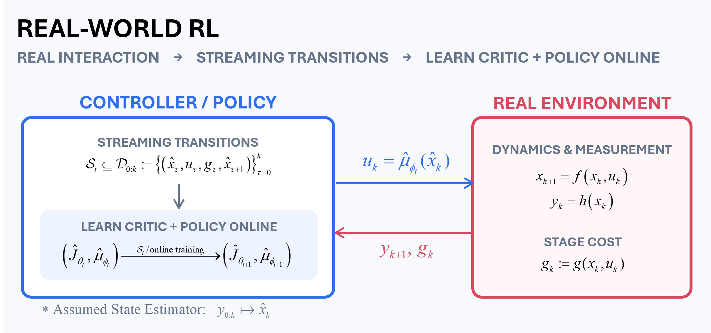
Real interactions generate streaming transitions that train both the critic and policy online
The environment returns measured transition records; an assumed state estimator converts the measurements into $\widehat x_k$ before the state-based transition enters $\mathcal S_t$. Without an estimator, $\widehat x_k$ is replaced by the information state $o_k$ defined below. Physical interaction is indexed by $k$, whereas network updates are indexed by $t$; the two clocks need not advance at the same rate. Here $k(t)$ is the latest physical-state sample available at learner update $t$, and $t(k)$ is the latest learner update available at physical step $k$. The figure abbreviates the available transition history for readability.
1. Problem definition
Online Learning-Based Optimal Control defines the desired policy through Bellman optimality. The broader Real-World RL Theme addresses the case in which its critic and, when explicitly parameterized, policy are learned from real closed-loop data. A representative approximate policy is
\[\widehat\mu_{\phi_t}(\widehat x) \approx \arg\min_{u\in\mathcal U(\widehat x)} \left\{ g(\widehat x,u) +\alpha\widehat J_{\theta_t} \!\left(\widehat f_{\psi_t}(\widehat x,u)\right) \right\}.\]$\widehat J_{\theta_t}$ is the critic and $\widehat\mu_{\phi_t}$ is the policy network, $\widehat f_{\psi_t}$ is a successor model with parameter $\psi_t$, and $0<\alpha<1$ is the discount factor. The expression above is model-based. Without a successor model, an observed transition provides a sample-based Q-factor target directly:
\[\widehat Q_t^{\mathrm{tar}}(\widehat x_k,u_k) := g(\widehat x_k,u_k)+ \alpha\widehat J_{\theta_t}(\widehat x_{k+1}).\]A learned Q-critic fits such targets over state–action pairs; model-free policy improvement then minimizes the learned Q-factor over $u$.
For the primary notation, a state estimator is assumed to supply the controller-facing state estimate. The real system then supplies a stream
\[d_k=(\widehat x_k,u_k,g_k,\widehat x_{k+1}), \qquad \mathcal D_{0:k(t)-1} := (d_0,\ldots,d_{k(t)-1}), \qquad \mathcal S_t\subseteq\mathcal D_{0:k(t)-1}.\]Here $g_k:=g(\widehat x_k,u_k)$ is the realized stage cost. Because a complete transition ending at the latest state sample $k(t)$ is indexed by $k(t)-1$, $\mathcal D_{0:k(t)-1}$ is the ordered collection of all completed transition records available to the learner. The update set $\mathcal S_t$ may contain the latest transition alone or selected prior transitions. Replay or minibatch training is optional rather than a defining assumption.
Without a state estimator, the problem is a partially observed setting. Then $\widehat x_k$ should be replaced by an observation or information state $o_k$: $o_k=y_k$ only when the current measurement is sufficient for control; otherwise $o_k$ should summarize an observation history, belief state, or learned latent state. The corresponding record is $d_k=(o_k,u_k,g_k,o_{k+1})$.
In an actor–critic realization, the selected update data train both learned objects:
\[\left( \widehat J_{\theta_t}, \widehat\mu_{\phi_t} \right) \xrightarrow[\mathcal S_t]{\mathrm{online\ training}} \left( \widehat J_{\theta_{t+1}}, \widehat\mu_{\phi_{t+1}} \right), \qquad u_k=\widehat\mu_{\phi_{t(k)}}(\widehat x_k).\]2. Why this problem matters
Many control-oriented RL methods are trained and evaluated primarily in simulation. Their deployed performance can then be limited by the sim-to-real gap: unmodeled dynamics, sensing imperfections, disturbances, and operating conditions absent from the simulator.
Learning directly from the real system can capture this missing information and continue improving when deployment reveals new operating conditions. Here, adaptability means accumulating and reusing experience to learn a critic and policy that remain useful over a declared task domain. It does not mean only tracking a local parameter change along the currently excited trajectory, as in an adaptive-control-like update.
3. Key challenges
- Limited and policy-dependent data: real transitions arrive sequentially and are correlated. Unlike simulator rollouts, they cannot be generated freely over the entire state–action domain.
- Local fit versus task-level learning: reducing loss on the latest trajectory can produce a local fit, forget earlier regimes, or repeatedly relearn the same task. The learned functions must retain broader task-relevant structure.
- Learning inside the closed loop: critic and policy change while the system is operating. Update time, action latency, stability, constraints, fallback behavior, and safety evidence must therefore be part of the learning problem.
4. A conventional approach — TD-error-based approximate policy iteration
One conventional approach is TD-error-based approximate policy iteration: fix the current policy, reduce its one-step temporal-difference error, and then perform policy improvement. For notational simplicity, this section writes $x_k$ as the state available to the controller; when an estimator is used, it is replaced by $\widehat x_k$. Here $\pi_i$ is the policy at policy-iteration step $i$.
\[\begin{aligned} \delta_k^{\pi_i} &= g(x_k,\pi_i(x_k)) +\alpha\widehat J^{\pi_i}(x_{k+1}) -\widehat J^{\pi_i}(x_k),\\ \widehat J^{\pi_i} &\xleftarrow{\mathrm{TD\ error\ reduction}} \operatorname{Fit}\!\left(\delta_k^{\pi_i}\right), \qquad \pi_{i+1} \leftarrow \operatorname{Greedy}\!\left(\widehat J^{\pi_i}\right). \end{aligned}\]This is a valid approximate-DP mechanism, but streaming data may make it adaptation-like: a small TD error on visited samples establishes sampled policy consistency, not task-wide Bellman optimality. Limited coverage can therefore yield episode- or trajectory-dependent critic parameters.
5. Current precursor — BOCO critic and constrained control learning
BOCO (Bellman Optimality via Constrained Optimization) first parameterizes the unknown optimal critic,
\[J^*(x)\approx\widehat J_\theta(x),\]and, at each selected update state, expresses the local Bellman minimization and equality as a finite-dimensional constrained optimization problem. This makes the local condition amenable to numerical KKT or primal–dual implementation:
\[\begin{aligned} F_k(u,\theta) &:= g(x_k,u)+ \alpha\widehat J_\theta\!\left(x_{k+1}(u)\right),\\ \delta_k(u,\theta) &:= F_k(u,\theta)-\widehat J_\theta(x_k), \end{aligned}\] \[\begin{aligned} \min_{u,\theta}\quad &F_k(u,\theta)\\ \mathrm{s.t.}\quad &\delta_k(u,\theta)=0,\\ &c_i(x_k,u)\le 0,\qquad i=1,\ldots,n_c. \end{aligned}\]Here $x_{k+1}(u)$ denotes the successor associated with candidate input $u$. Evaluating this quantity for arbitrary candidate inputs requires a declared control-usable model, simulator, or other counterfactual mechanism; one realized transition supplies the successor only for the input that was actually applied. The set $\mathcal U(x_k)$ contains admissible inputs, $n_c$ is the number of explicit inequality constraints, and $c_i$ is the $i$th such constraint. It may represent an actuator limit, a state-dependent feasibility condition, or a safety-related operating bound. These constraints can be added explicitly instead of being handled only by a penalty.
A global critic still requires accumulated streaming constraints, a declared collocation or update set, or another function-approximation condition; one local equality does not identify the complete value function.
The Lagrangian is
\[\mathcal L_k(u,\theta,\lambda) = F_k(u,\theta) +\lambda_\delta\delta_k(u,\theta) +\sum_{i=1}^{n_c}\lambda_i c_i(x_k,u), \qquad \lambda_i\ge 0.\]At online update $t$, the primal control, critic parameter, and multipliers can be updated conceptually as
\[\begin{aligned} u_k^{\mathrm{BOCO}} &\in \arg\min_{u\in\mathcal U(x_k)} \mathcal L_k(u,\theta_t,\lambda_t),\\ \theta_{t+1} &= \theta_t-\eta_{\theta,t} \nabla_\theta\mathcal L_k \!\left(u_k^{\mathrm{BOCO}},\theta_t,\lambda_t\right),\\ \lambda_{\delta,t+1} &= \lambda_{\delta,t} +\eta_{\delta,t}\, \delta_k\!\left(u_k^{\mathrm{BOCO}},\theta_t\right),\\ \lambda_{i,t+1} &= \left[ \lambda_{i,t} +\eta_{\lambda_i,t}\, c_i\!\left(x_k,u_k^{\mathrm{BOCO}}\right) \right]_+ . \end{aligned}\]Here $\lambda_t=(\lambda_{\delta,t},\lambda_{1,t},\ldots,\lambda_{n_c,t})$ collects the current multipliers, the $\eta$ terms are positive update step sizes, and $[\cdot]+$ projects each inequality multiplier onto the nonnegative orthant. The equality multiplier $\lambda\delta$ is unrestricted in sign. The physical state $x_k$ is embedded in $F_k$, $\delta_k$, $c_i$, and therefore $\mathcal L_k$.
Unlike TD-error reduction alone, BOCO keeps control minimization, critic consistency, and explicit constraints together. In the current formulation, $u_k^{\mathrm{BOCO}}$ is the primal actor decision and a separate policy-network parameter $\phi$ is not required. A future amortized policy network could be trained to reproduce this solution, but that is a distinct extension.
The current BOCO paper provides this formulation and constrained nonlinear simulation evidence. Formal stability, safety, broader task-domain learning, separate policy-network training, and real-system validation require additional assumptions and evidence.
6. Application domains
- Automatic tuning and calibration of control systems for electric drives and vehicle or mobility systems, using operational data to improve the deployed critic and controller.
- Controller learning in complex, unstructured real-world environments where a faithful simulator and exhaustive offline training data are difficult to obtain.
References
- H. Lee and K. Choi, “Constrained Optimization Formulation of Bellman Optimality Equation for Online Reinforcement Learning,” TechRxiv preprint, v1, 2025. Full text