Future Mobility Control Landscape
Core idea. Connected, automated, and electrified vehicles expand the information and decision scope of mobility control while adding coupled control and actuation degrees of freedom (DOFs) at mobility-system, vehicle, and component levels. Realizing this performance potential is naturally formulated as an optimal-control problem, but computational and information limitations often prevent its direct implementation. These shared barriers motivate learning-based optimal control.
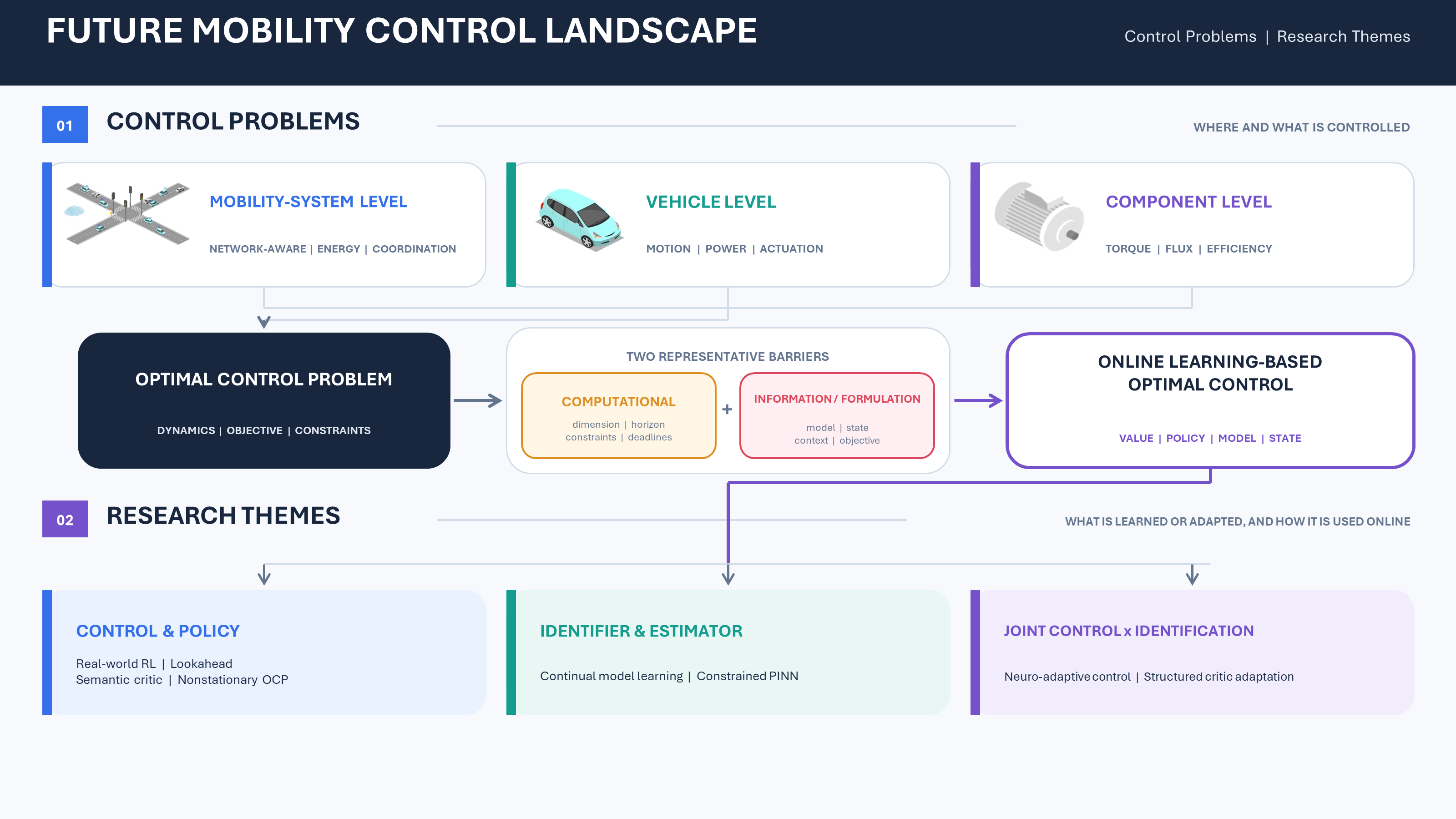
Future-mobility Control Problems at three levels lead through two representative barriers
and online learning-based optimal control to the MIC Lab Research Themes.
The two main axes organize where and what is controlled (Control Problems) and what is learned or adapted (Research Themes). Computational and information/formulation barriers motivate online learning-based optimal control as the bridge between them.
How to read this overview. Sections 1–3 establish the CAEV context, the common optimal-control principle, and the three control domains. Section 4 explains their shared implementation barriers and why they motivate the laboratory’s online learning-based control program. Section 5 maps the two complementary document families.
1. CAEVs and the need for multilevel optimal control
Future mobility is often described by CASE: connected, automated, shared, and electrified mobility. This control landscape focuses on connected, automated, and electrified vehicles (CAEVs). Shared mobility remains relevant when demand, fleets, or shared resources enter a mobility-system problem, but it does not define a separate physical control level here.
The three CAEV characteristics change control in complementary ways:
- Connected: broadens the available information to include route, traffic, infrastructure, other agents, pedestrians, and cloud services.
- Automated: transfers more planning, coordination, and actuation decisions to feedback controllers.
- Electrified: adds coupled energy and thermal states, multiple power sources, distributed electric actuators, and fast electrical commands.
These characteristics create control opportunities at three levels:
- Mobility-system level: use route, traffic, infrastructure, mission, or connected-agent information for trip-scale energy and thermal management or multi-vehicle coordination.
- Vehicle level: coordinate onboard drive, brake, steering, or suspension actuators.
- Component level: control device-level variables such as motor voltage, current, flux, and torque.
Connected, automated, and electrified functions contribute across all three levels rather than mapping one-to-one to them. Across the levels, CAEVs broaden the information available to the controller, enlarge the set of coupled decisions, and add control and actuation degrees of freedom (DOFs).
For example, a connected electrified vehicle (xEV) can use previews of road grade, signal timing, traffic, weather, or charging opportunities to improve present energy and thermal decisions over the trip. Multiple connected vehicles can additionally coordinate speed, spacing, lane selection, or intersection passage. Optimal control provides a common formulation for using this information and the available control DOFs to balance performance and constraints.
2. Optimal control as a common decision principle
The details change across applications, but the basic optimal-control question is the same:
| Conceptual problem definition | |
|---|---|
| Find | An admissible control input, control sequence, or feedback policy |
| To minimize | A performance index encoding energy use, travel time, safety penalties, motion error, discomfort, or component loss |
| Subject to | System dynamics, physical and safety constraints, actuator limits, environmental conditions, and the information available to the controller |
The exact states, inputs, costs, models, and constraints depend on the control level and application; Section 3 specifies those differences.
3. Three mobility control problem domains
The three levels are classified first by the primary performance objective and the boundary of the coupled decisions and information—not merely by where an actuator is physically located. Physical location and time scale are secondary descriptors. The same electric motor can therefore support component-level torque control, vehicle-level actuator allocation, and mobility-system-level energy management.
Mobility-System-Level Optimal Control
This domain uses route, traffic, infrastructure, ambient, mission, or connected-agent information beyond the local vehicle state. It includes a single xEV using such context for predictive or infinite-horizon energy and thermal management, as well as multiple vehicles coordinating through shared information. A traffic network is therefore one information source within the broader mobility system; multiple vehicles are an important case, but not the definition of this level. Energy management belongs here when route or mobility context and long-horizon coupling define the problem; a local power-split problem using only onboard variables can instead be vehicle-level.
Vehicle-Level Optimal Control
This domain coordinates control and actuation DOFs contained in the whole vehicle. Representative decisions include propulsion and braking allocation, torque vectoring, four-wheel independent drive or steering, and steering–suspension coordination. The objectives may combine motion, stability, safety, comfort, and efficiency subject to tire, actuator, power, and vehicle-dynamics constraints.
A related deployment problem is Automatic Controller Calibration: gains, maps, cost weights, filters, thresholds, or learned parameters of vehicle-motion controllers are adjusted to reproduce the intended behavior across maneuvers and operating conditions. The vehicle-level page treats this as an outer-loop workflow surrounding the physical control problem.
Component-Level Optimal Control
This domain exploits fast device-level control DOFs. A representative problem is optimal torque production in a synchronous machine through voltage or inverter-switching decisions that shape current and flux while respecting electrical, magnetic, thermal, inverter, and sampling constraints.
The same workflow appears at the component level when current-, torque-, speed-, position-, estimator-, or solver-related parameters must be adjusted across machine and operating conditions. In both the vehicle and component domains, calibration is a deployment and lifecycle workflow rather than a fourth physical control level.
4. Why direct optimal control is difficult — and what learning contributes
Implementing the principle in Section 2 requires both finding the optimal input or policy within the available computation time and having the model, state, context, objective, constraints, and transition information needed to define and evaluate the decision. Two difficulties recur across all three control levels:
- Computational difficulty: high-dimensional state and action spaces, long horizons, hybrid decisions, nonlinear constraints, coupled agents, and short control deadlines can make exact policy computation or repeated online optimization impractical.
- Information and formulation limitations: the model, state, context, objective, constraints, or transition law needed to define and evaluate the decision may be incomplete, uncertain, indirectly measured, or changing. Limited real-world data can further restrict identification and validation.
The first difficulty means that an exact optimal decision may be too expensive even when the required information is available. The second means that the decision problem or its evaluation is incomplete, unreliable, or nonstationary. Many mobility problems contain both.
These barriers motivate learning-based optimal control. When exact decision computation is too expensive, a learned value or policy—or a learned object combined with tractable online optimization—can approximate the optimal decision. When the required information is incomplete or changing, the relevant model, state, context, or representation can instead be estimated, learned, or updated.
Within this broad class, the MIC Lab program emphasizes the online realization of learning-based optimal control, including online learning when deployed learned objects must adapt. Current measurements, context, forecasts, and constraints may support online estimation, decision improvement, or parameter learning; online learning is reserved for the last case. The common formulation and eight Research Themes are developed in Online Learning-Based Optimal Control.
5. Document map — two complementary views
The two views are complementary rather than one-to-one. A project may involve one or more physical Control Problem domains and draw on one or more Research Themes.
| View | Organizing question | Overview and child pages |
|---|---|---|
| Mobility Control Problem Domains | Where and what is controlled? | Overview (00): Future Mobility Control Landscape Domain pages (01–03): 01 · Mobility-System-Level Optimal Control 02 · Vehicle-Level Optimal Control 03 · Component-Level Optimal Control |
| Learning-Based Control Research Themes | Which bottleneck and learned object are addressed, and how are they used online? | Overview (00): Online Learning-Based Optimal Control Theme pages (01–08): 01 · Real-World RL 02 · Online Multistep Lookahead 03 · Semantic Critic Learning 04 · Nonstationary Infinite-Horizon OCP 05 · Continual Model Learning 06 · Constrained PINN 07 · Neuro-Adaptive Control 08 · Structured Critic Adaptation |