Vehicle-Level Optimal Control
Core idea. Vehicle-level optimal control maps driver or automated-driving commands into coordinated propulsion, braking, steering, and suspension actions. Automatic calibration is a coupled deployment workflow that adjusts gains, maps, cost weights, and learned parameters to reproduce the intended agility–stability balance across real operating conditions under declared safety checks.
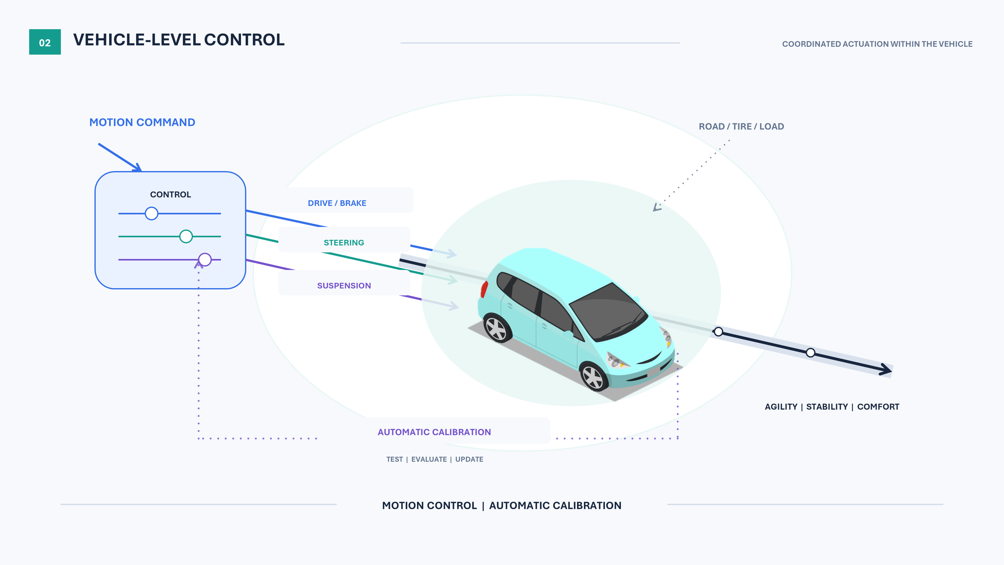
A motion command is realized through coordinated drive, brake, steering, and suspension actuation,
while measured vehicle response supports automatic calibration.
Vehicle-level control coordinates onboard actuators to shape whole-vehicle motion. Automatic calibration is a coupled deployment workflow rather than a separate physical control level.
1. Scope: coordinated control within the vehicle
Future Mobility Control Landscape defines vehicle-level control by where the primary performance objective and coupled decisions are formed. The boundary is the whole vehicle: driver or automated-driving commands and onboard measurements enter the controller, and the controller coordinates onboard actuators to shape the resulting motion.
Representative elements are
| Role | Examples |
|---|---|
| Commands and context | desired speed, path, yaw or acceleration response, vehicle mode, payload, and estimated road condition |
| Decision state | longitudinal and lateral motion, yaw, sideslip, roll or heave, wheel motion, tire-force utilization, and actuator states |
| Control inputs | distributed drive or brake torque, front/rear or individual-wheel steering, and active-suspension force |
| Performance | path and motion tracking, agility, stability, safety, ride comfort, efficiency, and actuator smoothness |
| Constraints | tire-force capacity, vehicle stability envelope, actuator magnitude/rate, power, comfort, and electronic control unit (ECU) execution limits |
This scope includes controllers acting through one or several actuator families. At its broadest realization, it includes integrated chassis control, which coordinates longitudinal, lateral, and vertical vehicle motion through propulsion or braking, steering, and suspension actuators. The vehicle-level domain is not restricted to such a fully integrated architecture: a steering-only or torque-vectoring controller also belongs when its objective is whole-vehicle motion.
The subject is established, but expanding vehicle actuation changes the research question. Distributed electric drive, independent steering, braking, and active suspension provide more ways to generate the same net force and moment, while all of them compete for coupled tire and actuator capacity. The challenge is therefore not merely to add another feedback loop. It is to use the available actuation degrees of freedom coherently under uncertain tire–road interaction and to realize a desired vehicle character on the real vehicle.
Local power-source allocation using only onboard state and demand is formally vehicle-level. MIC Lab’s main energy-management work is nevertheless treated under mobility-system-level control because route, traffic, infrastructure, mission, and long-horizon context materially determine the decision. This page therefore focuses on whole-vehicle motion and its calibration workflow.
2. Representative control problem and deployment workflow
| Role | Main decisions | Main objective |
|---|---|---|
| Physical control problem — Vehicle motion control | coordinate the available traction, braking, steering, and suspension actions over the vehicle | produce the commanded motion while balancing agility, stability, comfort, efficiency, and tire/actuator margins |
| Cross-cutting deployment workflow — Automatic calibration of vehicle-motion controllers | select gains, maps, cost weights, filters, thresholds, or critic/policy parameters | reproduce the intended behavior across speed, maneuver, road, load, tire, and vehicle conditions with fewer manual real-vehicle iterations |
These are coupled stages in one deployment workflow, not separate physical control levels. Motion control determines the action for a fixed design and calibration; the outer-loop calibration workflow in Section 3.2 adjusts only declared parameters against measured vehicle response and an evaluable target behavior.
3. Vehicle motion control and its calibration workflow
3.1 Vehicle motion control
Let $x_k$ denote the vehicle, wheel, and actuator state; $u_k$ the coordinated actuator command; $\xi_k^{\mathrm{cmd}}$ the driver or automated-driving command; and $\eta_k$ the control-relevant operating condition. The latter may include road friction, tire condition, mass and load distribution, or another slowly changing physical context:
\[\begin{aligned} x_{k+1} &= f(x_k,u_k;\eta_k)+w_k,\\ y_k &= h(x_k)+v_k . \end{aligned}\]Here $y_k$ is the measured output, $h$ the measurement map, and $w_k$ and $v_k$ process and measurement disturbances, respectively. Tire force, sideslip, friction, and some vertical-load or actuator states may not be measured directly, so the controller generally uses $\widehat x_k$ and $\widehat\eta_k$ supplied by an estimator or identifier.
At physical time $k$, a representative predictive motion-control problem is
\[\begin{aligned} U_k^\star \in \arg\min_{U_k}\quad& \sum_{j=0}^{H-1} \alpha^j \ell_{\mathrm{mot}} \!\left( x_{j\mid k}, u_{j\mid k}, \xi_{j\mid k}^{\mathrm{cmd}};q \right) + \alpha^H V_{\mathrm f}(x_{H\mid k})\\ \mathrm{s.t.}\quad& x_{0\mid k}=\widehat x_k,\\ & x_{j+1\mid k} = f_{\mathrm{use}} \!\left( x_{j\mid k},u_{j\mid k};\widehat\eta_k \right), \quad j=0,\ldots,H-1,\\ & x_{j\mid k} \in \mathcal X \!\left(\widehat\eta_k\right), \quad j=0,\ldots,H,\\ & u_{j\mid k} \in \mathcal U \!\left(x_{j\mid k};\widehat\eta_k\right), \quad j=0,\ldots,H-1. \end{aligned}\]$U_k=(u_{0\mid k},\ldots,u_{H-1\mid k})$ is the candidate actuator sequence, $H$ is the horizon, and $0<\alpha\le 1$ is the finite-horizon discount factor. $f_{\mathrm{use}}$ is the declared prediction model, $V_{\mathrm f}$ the terminal value, and $q$ the stage-cost weight vector. The feasible sets $\mathcal X$ and $\mathcal U$ can encode a tire-force or friction envelope, vehicle-stability bounds, actuator magnitude and rate limits, power limits, and ride or safety constraints. $H$ may be one for a static allocation or longer for predictive motion control.
A schematic stage cost is
\[\ell_{\mathrm{mot}} = q_{\mathrm{trk}}\ell_{\mathrm{trk}} + q_{\mathrm{ag}}\ell_{\mathrm{agility}} + q_{\mathrm{st}}\ell_{\mathrm{stability}} + q_{\mathrm{com}}\ell_{\mathrm{comfort}} + q_u\ell_{\mathrm{effort}} .\]This decomposition is not a universal definition of vehicle feel. The loss terms select measurable proxies, while the weight vector $q$ determines their trade-off. Both the model used by the optimizer and the cost structure used to judge the response must therefore be validated on the real vehicle.
The deployed controller may be an online optimizer, a conventional controller with calibrated maps, or a learned policy. They can be represented uniformly as
\[u_k = \mu_{\rho} \!\left( \widehat x_k, \xi_k^{\mathrm{cmd}}, \widehat\eta_k \right),\]where $\rho$ collects the quantities exposed to calibration: gains, maps, filters, thresholds, optimal-control weights, or policy parameters.
3.2 Automatic calibration during implementation and validation
A representative model-based workflow produces an initial calibration $\rho_0$. After deployment to a vehicle ECU, engineers repeat real-vehicle tests, quantitative evaluation, driver assessment, and manual calibration:
\[\text{model-based design} \rightarrow \text{ECU deployment} \rightarrow \text{vehicle test} \rightarrow \text{evaluation} \rightarrow \text{manual recalibration}.\]Automatic calibration seeks to make this outer loop systematic and sample-efficient. Let $n$ index a real or accepted high-fidelity calibration trial, $\chi_n$ its operating context, and $\tau_n(\rho_n)$ the measured closed-loop trajectory under calibration $\rho_n$. The trial produces quantitative motion metrics $m_n$ and, when used, a declared driver or test-engineer assessment $s_n$. Define
\[d_n^{\mathrm{cal}} := \left( \chi_n,\rho_n,\tau_n,m_n,s_n \right), \qquad \mathcal D_{0:n}^{\mathrm{cal}} := \left\{ d_i^{\mathrm{cal}} \right\}_{i=0}^{n}.\]The ideal calibration objective is the expected evaluation loss over the declared operating-condition distribution $\mathcal P_{\mathrm{op}}$:
\[\mathcal L_{\mathrm{cal}}(\rho) := \mathbb E_{\chi\sim\mathcal P_{\mathrm{op}}} \left[ \mathcal L_{\mathrm{eval}} \!\left( \tau(\mu_\rho;\chi), s_{\mathrm{des}} \right) \right],\]where $s_{\mathrm{des}}$ denotes the intended vehicle character or preference. Because this expectation cannot be evaluated freely on a real vehicle, a data-driven tuning step uses the accumulated trials to select the next admissible calibration:
\[\rho_{n+1} \in \arg\min_{\rho\in\mathcal P_n^{\mathrm{adm}}} \widehat{\mathcal L}_{\mathrm{cal},n} \!\left( \rho;\mathcal D_{0:n}^{\mathrm{cal}} \right).\]$\widehat{\mathcal L}{\mathrm{cal},n}$ is a data-supported estimate or surrogate of $\mathcal L{\mathrm{cal}}$, and $\mathcal P_n^{\mathrm{adm}}$ is the candidate set admitted at trial $n$ by declared parameter bounds, pre-test safety checks, and controller acceptance logic. $\mathcal L_{\mathrm{eval}}$ can combine quantitative motion metrics with a preference error only after the latter has been converted into an evaluable rating, label, comparison, or learned surrogate. Actuator and state constraints, worst-case ECU execution time, fallback behavior, and the number and coverage of safe real trials remain part of the calibration protocol even when they are not all written inside this compact argmin.
This formulation does not require every production parameter to be learned. The calibration object $\rho$ should include only parameters whose role, admissible range, and verification procedure have been declared.
4. Why vehicle motion control and calibration are difficult
-
Information and formulation limitations: tire forces are nonlinear, saturating, coupled, and only partly observed; friction, tire condition, temperature, payload, and maneuver further change the relevant dynamics. Agility and stability can be quantified through selected proxies, but their relation to perceived handling quality or the intended vehicle character is not unique. The controller must therefore identify the required state and model while expressing subjective assessment through measurable metrics, ratings, comparisons, or another explicit teaching signal. Real calibration data arrive sequentially and cannot be explored freely.
-
Computational difficulty: a moderate-order, fixed-model model predictive controller (MPC) can be practical. The burden grows with nonlinear coupled dynamics, multiple actuators, tire and safety constraints, longer-horizon effects, and online learning. These operations must fit within ECU memory, latency, and verification limits.
The information and formulation barrier determines what must be identified and what performance should mean; computational difficulty limits how much of the resulting control and learning problem can be performed online.
5. Two research questions
- Representation under uncertainty: How can control-oriented vehicle and tire dynamics, latent motion states, and the desired agility–stability behavior be represented accurately across changing road, tire, load, maneuver, and vehicle conditions?
- Real-time policy and calibration: How can the coupled motion policy and its calibration be computed or learned within ECU and real-test limits while preserving safety, prior knowledge, and performance over the declared operating domain?
6. MIC Lab approach and connections to research themes
The two research questions can be approached through model/state learning, approximate optimal control, and safe real-world policy improvement. These mechanisms may be used separately or combined; no single research theme is assumed to solve the complete vehicle problem.
6.1 Model and state uncertainty: continual control-oriented model learning
Fast observers and adaptive identifiers can estimate the current condition, but minimizing the latest residual does not ensure that the learned model remains accurate across the vehicle’s operating domain. Continual Model Learning instead adds new tire and vehicle behavior while retaining control-relevant behavior learned in earlier conditions. When the required state is latent, state and model estimation can be coupled while a retention term preserves selected prior function behavior. The result must be evaluated by state-estimation quality, multistep tire/vehicle prediction, and downstream control performance—not only one-step prediction error.
6.2 Computational difficulty: approximate DP and structured critic reuse
Online Learning-Based Optimal Control connects the vehicle problem to approximate dynamic programming (ADP): an expensive long-horizon solution can be represented by an approximate critic or policy and reused online.
When a compact operating parameter $\eta$ captures changes such as road friction, load, or tire condition, Structured Critic Adaptation provides a candidate bridge between identification and policy improvement. The identified condition reconfigures a stored value structure before policy improvement, avoiding repeated full critic or policy learning across recurring conditions. This does not make every fixed MPC solve faster by itself.
Online Multistep Lookahead can then use the fixed or reconfigured critic as a terminal value while a short online horizon resolves the current nonlinear dynamics, tire limits, and actuator constraints. If repeated optimization remains too expensive, its state-to-solution map can be learned as a policy for faster ECU execution.
6.3 Automatic calibration: constrained Real-World RL
Real-World RL is a candidate method for the automatic-calibration problem in Section 3. It can use streaming real transitions to improve a critic and, when declared, policy or controller parameters, reducing dependence on a simulator that omits control-relevant tire, sensing, actuator, or driver effects. The intended goal is reusable task-domain learning across the declared operating conditions, not only a trajectory-local adaptive fit.
The reward or cost must still be specified. Quantitative agility, stability, comfort, effort, and safety metrics can provide its primary terms; driver or test-engineer assessment can be used only after it is converted into a declared learning signal. Explicit constraints, guarded updates, fallback control, test acceptance, and closed-loop evidence remain necessary for real-vehicle learning. Real-World RL is therefore a possible implementation of automatic calibration, not a synonym for the calibration problem itself.
6.4 Supporting research connections
| Research theme | Possible role in this control domain |
|---|---|
| Semantic Critic Learning | Convert scenario descriptions, driver comparisons, or other contextual feedback into an auxiliary critic-learning signal. This is a candidate extension, not a substitute for a declared control objective. |
| Neuro-Adaptive Control | Approximate an uncertain ideal motion-control law or residual directly and adapt it under closed-loop and input constraints. Its trajectory-local adaptation role should be distinguished from global model retention and task-domain calibration. |
| Constrained PINN | Learn a physics-consistent tire or vehicle field/model while imposing selected boundary, initial, constitutive, or feasibility conditions explicitly. |
| Nonstationary Infinite-Horizon OCP | Address cases in which changing operating context, constraints, or desired behavior can prevent one stationary critic from representing the exact long-run optimum. An approximate or robust stationary critic may remain useful under stated conditions, so this Theme is not required for every motion controller. |