Continual Model Learning
Core idea. Continual Model Learning incorporates newly observed system behavior into a learned dynamics model while retaining control-relevant behavior learned in earlier operating regions. When the physical state is not directly measured, the state trajectory and model can be learned jointly.
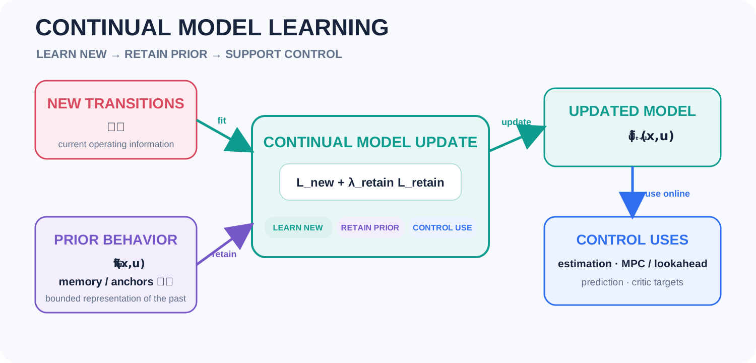
Continual model learning fits new data while retaining prior model behavior
Physical interaction is indexed by $k$, whereas learner updates are indexed by $t$; the two clocks need not advance at the same rate. $\widehat\psi_t$ denotes the model parameter available before update $t$, and $\widehat\psi_{t+1}$ denotes the updated parameter.
1. Problem definition
Online Learning-Based Optimal Control requires decision-state and successor information for Bellman-based control. Continual Model Learning addresses the identifier/estimator-side problem: learn a dynamics model from new real measurements without losing earlier model behavior still needed by the estimator or controller.
Consider
\[x_{k+1}=f(x_k,u_k,w_k), \qquad y_k=h(x_k)+v_k,\]where $x_k$, $u_k$, and $y_k$ are the state, control input, and measurement; $f$ and $h$ are the state-transition and measurement maps; and $w_k$ and $v_k$ represent process and measurement uncertainty. Unless a different stochastic predictor is declared, the learned one-step target is the conditional mean
\[\overline f(x,u) := \mathbb E[x_{k+1}\mid x_k=x,u_k=u] \approx \widehat f_{\widehat\psi_t}(x,u).\]The primary continual-learning scope is coverage expansion for a fixed underlying predictor $\overline f$: new operating regions are added while selected prior function behavior is retained. Genuine physical drift is a different case. If the same $(x,u)$ acquires a different successor law because of temperature, aging, load, or another condition, that condition should be represented explicitly, for example by $\overline f(x,u;\eta)$, or handled by a declared tracking/forgetting rule. Blind retention can otherwise preserve obsolete behavior.
When both state and model are unknown, the basic identification principle is measurement–dynamics consistency:
\[\left(x_{0:k}^{\star},\psi^{\star}\right) \in \arg\min_{x_{0:k},\psi} \left\{ \mathcal L_{\mathrm{meas}}(x_{0:k};y_{0:k}) + \mathcal L_{\mathrm{dyn}}(x_{0:k},\psi;u_{0:k-1}) \right\}.\]For example, quadratic measurement and dynamics residuals are
\[\begin{aligned} \mathcal L_{\mathrm{meas}}(x_{0:k};y_{0:k}) &= \sum_{i=0}^{k} \left\|y_i-h(x_i)\right\|_{W_y}^{2},\\ \mathcal L_{\mathrm{dyn}}(x_{0:k},\psi;u_{0:k-1}) &= \sum_{i=0}^{k-1} \left\| x_{i+1}-\widehat f_{\psi}(x_i,u_i) \right\|_{W_x}^{2}, \end{aligned}\]where $W_y\succeq0$ and $W_x\succeq0$ weight the measurement and dynamics residuals, respectively. An online implementation evaluates these losses over a recent window rather than the entire trajectory.
Real measurements form the stream
\[d_k=(y_k,u_k,y_{k+1}), \qquad \mathcal D_{0:k(t)-1} := (d_0,\ldots,d_{k(t)-1}), \qquad \mathcal S_t\subseteq\mathcal D_{0:k(t)-1}.\]Here $k(t)$ is the latest measurement/state index available at learner update $t$. The set $\mathcal S_t$ may contain only the latest completed transition or a short selected history. If the state is directly measured, replace $y_k$ by $x_k$ and the problem reduces to model learning alone. Otherwise, the latent state trajectory and model parameters must be estimated jointly, or a separate estimator must supply $\widehat x_k$.
2. Why this problem matters
A model learned once offline may become incomplete as a mobility system visits new loads, temperatures, road conditions, aging states, or operating regions. Online system identification can reduce the residual on the newest trajectory, but the updated function may no longer represent regions learned earlier.
This distinction matters because a controller does not query the model only at the latest sample. State estimators, MPC or lookahead optimization, and critic targets may evaluate it over many control-relevant states and inputs. Continual learning therefore seeks both new-region fit and prior-function retention, rather than only a small current residual.
3. Key challenges
- Limited and policy-dependent data: real transitions arrive sequentially along the deployed closed-loop trajectory and do not freely cover the full state–input domain.
- New learning versus prior-function retention (the stability–plasticity trade-off): the learner must incorporate newly observed behavior without overwriting earlier behavior that remains relevant.
- State–model coupling: when $x_k$ is latent, state-estimation error and model error can explain the same residual and must be separated under suitable observability and excitation conditions.
- Control-relevant online learning: memory, update time, multistep error, model acceptance, and the effect of each update on downstream control matter in addition to one-step prediction loss.
4. A conventional approach — recent-data residual minimization
One conventional online-identification approach fits the model to the latest transition or a short recent window. For notational simplicity, assume here that the state is available; $x_j$ is replaced by $\widehat x_j$ when a separate estimator is used:
\[\begin{aligned} \widehat\psi_{t+1} &\approx \arg\min_{\psi} \mathcal L_{\mathrm{new}}(\psi;\mathcal S_t),\\ \mathcal L_{\mathrm{new}}(\psi;\mathcal S_t) &:= \sum_{j\in\mathcal I_t} \left\| x_{j+1}-\widehat f_{\psi}(x_j,u_j) \right\|_{W_x}^{2}. \end{aligned}\]$\mathcal I_t$ indexes the recent transitions admitted to update $t$. This update is useful for reducing current residuals, especially when the physical dynamics truly change. Under limited excitation, however, it becomes a trajectory-local online-identification update: it fits the currently visited region but does not explicitly preserve model behavior learned in earlier regions.
Tracking a genuinely changing model and retaining knowledge over an expanding task domain are therefore different objectives and should be evaluated separately.
5. Research direction — function-retaining continual learning
A continual formulation augments current measurement–dynamics consistency with explicit retention of the previously learned function. Let $k_t:=k(t)$ be the newest physical sample available at learner update $t$, and let $M$ be the estimation-window length. The set $\mathcal S_t$ supplies the transitions selected to fit newly observed behavior, whereas $\mathcal M_t={(\bar x_\ell,\bar u_\ell)}_{\ell=1}^{m_t}\subseteq\mathcal X\times\mathcal U$ is a bounded set of state–input anchors selected to retain prior model behavior. An anchor may be derived from a transition in $\mathcal S_t$, but $\mathcal M_t$ can additionally contain earlier stored points with pseudo-targets generated from the pre-update model:
\[\begin{aligned} \left( \widehat x_{k_t-M:k_t}, \widehat\psi_{t+1} \right) \approx \arg\min_{x_{k_t-M:k_t},\psi} \Big\{& \mathcal L_{\mathrm{meas},t}(x;\mathcal S_t) + \mathcal L_{\mathrm{dyn},t}(x,\psi;\mathcal S_t)\\ &+ \lambda_{\mathrm{retain}} \mathcal L_{\mathrm{retain}} \!\left( \widehat f_{\psi}, \widehat f_{\widehat\psi_t}; \mathcal M_t \right) \Big\}. \end{aligned}\]Here $\mathcal L_{\mathrm{meas},t}$ and $\mathcal L_{\mathrm{dyn},t}$ are the residual losses defined in Section 1, evaluated on $\mathcal S_t$. In a recent-window implementation, $\mathcal S_t={d_j\mid j=k_t-M,\ldots,k_t-1}$ supports the state and measurement window ending at $k_t$. The retention weight satisfies $\lambda_{\mathrm{retain}}\ge0$.
For example, functional retention over a bounded anchor set $\mathcal M_t$ can be written as
\[\mathcal L_{\mathrm{retain}} = \frac{1}{|\mathcal M_t|} \sum_{(\bar x,\bar u)\in\mathcal M_t} \left\| \widehat f_{\psi}(\bar x,\bar u) - \widehat f_{\widehat\psi_t}(\bar x,\bar u) \right\|_{W_r}^{2}.\]This expression assumes $|\mathcal M_t|>0$ and a positive-semidefinite weight $W_r\succeq0$. If no anchors are retained, the retention term is omitted.
The first two losses explain current measurements and dynamics; the last loss retains selected input–output behavior of the model available before the update. If $x_k$ is measured, remove the state-trajectory decision and $\mathcal L_{\mathrm{meas},t}$. The retention weight and anchor set define a design tradeoff; they do not guarantee global accuracy or eliminate forgetting.
Candidate mechanisms include a small representative replay set, local or RBF activation, pseudo-data generated from the previous model, and functional regularization. These are candidate directions, not achieved MIC Lab results.
Future evidence should compare recent-only fitting, bounded-memory retention, and full replay using new-region error, return-to-prior-region error, multistep prediction, estimator error, downstream control performance, memory, and update time.
6. Application domains
- Continual calibration of vehicle, electric-drive, energy-management, and thermal-system models across operating regions and explicitly represented load, temperature, or aging conditions.
- Control-oriented model learning for state estimation, MPC, online lookahead, and critic targets, where the model must remain useful beyond the latest trajectory.
- Model learning in complex real environments where complete offline data and repeated full retraining are impractical.