Online Learning-Based Optimal Control
Core idea. MIC Lab starts from one optimal-control problem. Bellman optimality gives the exact decision principle. Learning makes that principle implementable when exact computation, the dynamics, or the physical state is unavailable.
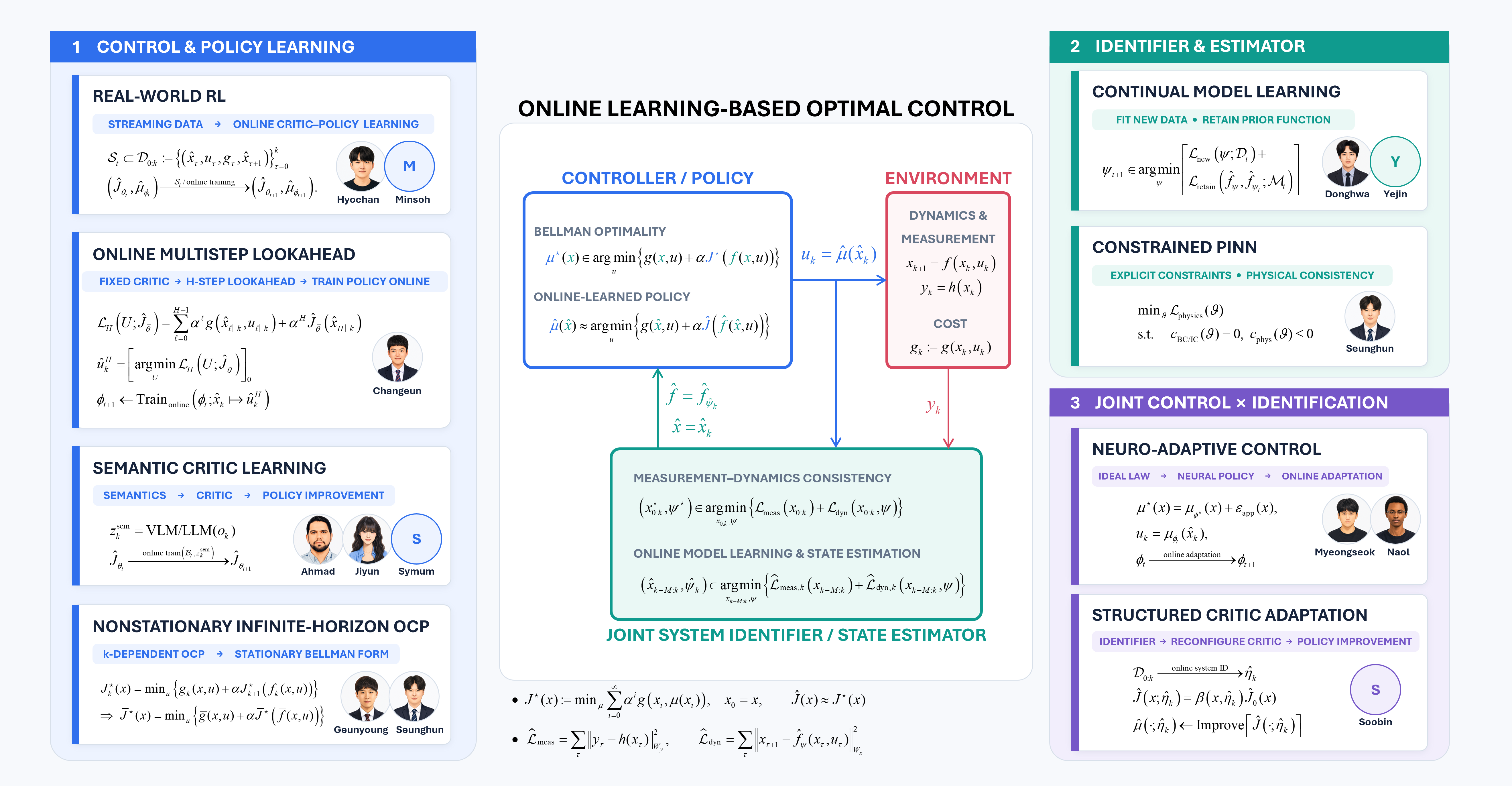
MIC Lab learning-based control research themes:
a common online learning-based optimal-control framework surrounded by eight research themes
MIC Lab Learning-Based Control Research Themes. The center presents the common optimal-control, environment, identification, and estimation framework. The surrounding cards organize eight research themes by the learned object and its role in the closed loop.
How to read this overview. Sections 1–3 establish the common optimal-control and Bellman reference. Sections 4–6 organize the three learning roles. Section 7 summarizes the boundary among all eight Research Themes. Section 8 states the scope and evidence requirements.
1. The optimal-control problem
The environment supplies dynamics, measurements, and stage cost:
\[\begin{aligned} x_{k+1} &=f(x_k,u_k,w_k),\qquad y_k=h(x_k)+v_k,\\ g_k&:=g(x_k,u_k). \end{aligned}\]$x_k$, $u_k$, $w_k$, $y_k$, and $v_k$ denote the state, control input, process disturbance, measurement, and measurement noise; $f$, $h$, and $g$ are the dynamics, measurement map, and stage cost. Thus $g_k$ is the realized scalar stage cost at step $k$.
To obtain the best long-horizon performance in this environment—equivalently, to minimize the stated cost—the controller is determined by solving
\[\begin{aligned} \mu^* &\in \arg\min_{\mu}\; \mathbb E_{\mu,\,x_0\sim p_0}\!\left[ \sum_{k=0}^{\infty} \alpha^k g\!\left(x_k,\mu(x_k)\right) \right],\\ \text{s.t.}\qquad u_k&=\mu(x_k)\in\mathcal U(x_k), \qquad 0<\alpha<1. \end{aligned}\]Here $p_0$ is the declared initial-state distribution; a fixed initial state is represented by a point mass at that state. The expectation is over this initial condition and any declared stochastic dynamics or disturbances.
When $x_k$ is not measured, an estimated state or another sufficient decision state must replace it in the implemented controller; Section 5 explains that part of the loop.
2. Bellman optimality gives the solution principle
The optimal value function is the minimum cost-to-go from state $x$:
\[J^*(x) := \inf_{\mu} \mathbb E_{\mu}\!\left[ \left. \sum_{j=0}^{\infty} \alpha^j g\!\left(x_j,\mu(x_j)\right) \right|x_0=x \right].\]For a stationary discounted problem with a valid Markov decision state, it satisfies
\[\begin{aligned} J^*(x) &= \min_{u\in\mathcal U(x)} \left\{ g(x,u)+\alpha\, \mathbb E[J^*(x^+)\mid x,u] \right\},\\ \mu^*(x) &\in \arg\min_{u\in\mathcal U(x)} \left\{ g(x,u)+\alpha\, \mathbb E[J^*(x^+)\mid x,u] \right\}. \end{aligned}\]$x^+$ denotes the successor state associated with the current state and action.
Dynamic programming (DP) uses this recursion to evaluate a policy and improve the decision rule. Thus, $J^*$ is the exact value function, and the minimizing decision defines the exact optimal policy. The next section explains how learning makes these Bellman objects—and the information required to compute them—available in practice.
3. Why learning-based control is needed
- Computational difficulty: even with usable state and dynamics, high-dimensional DP, long-horizon optimization, and constraint handling may be too expensive for exact offline or online solution.
- Information and formulation limitations: the dynamics $f$, current state $x_k$, disturbance law, operating context, objective, or constraints needed by the Bellman problem may be incomplete, only indirectly measured, or changing during operation.
Learning-based control makes the Bellman principle implementable by learning the objects or information that its exact solution requires. Within this broader framework, the Controller & Policy lane is naturally viewed as approximate dynamic programming (ADP): it approximates the Bellman value or Q-factor and/or the policy produced by Bellman improvement.
Learning a dynamics model or estimating the state is not, by itself, ADP. The Identifier & Estimator lane supplies missing decision-state or successor information that ADP—or another control optimizer—can use. The Joint Control × Identification lane couples these two roles.
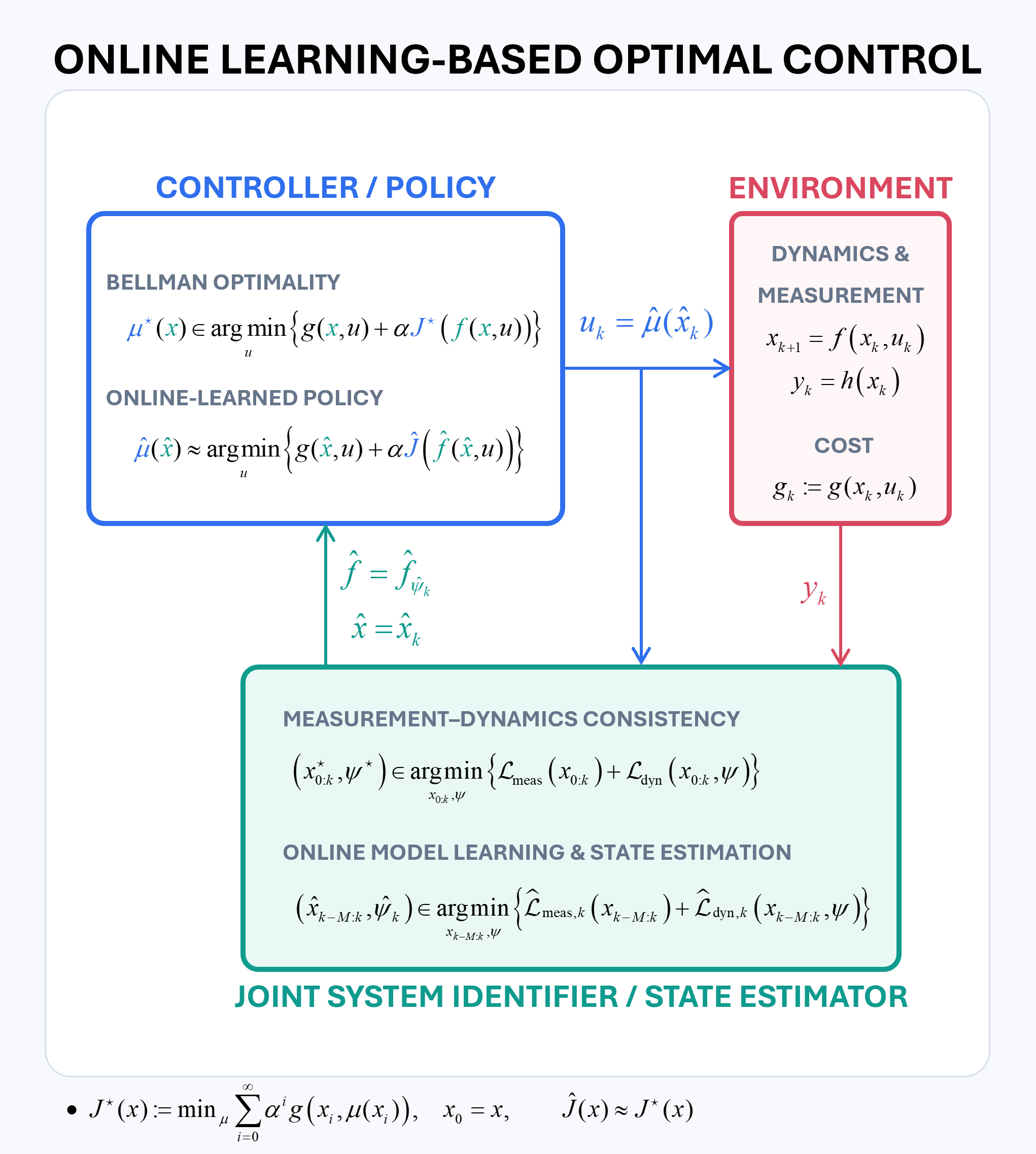
Bellman optimality, the environment, and joint online model learning and state estimation form the learning-based control loop.
The diagram suppresses some function-parameter subscripts for readability. Section 4 writes the learned critic, policy, and model as $\widehat J_{\theta_t}$, $\widehat\mu_{\phi_t}$, and $\widehat f_{\psi_t}$.
4. Controller & policy — learn a critic, a policy, or both
Section 2 gives the exact Bellman recursion, and Section 3 identifies its control-side approximation as ADP. This lane implements that idea by learning a critic, a policy, or both, while treating state and successor information as measured, estimated in Section 5, or sampled from the environment. The Themes below differ mainly in which Bellman object is learned online and which object is fixed or reformulated.
A representative model-based realization trains a policy to reproduce the action obtained from a learned critic and model. Physical time is indexed by $k$, optimizer updates by $t$, and $t(k)$ denotes the parameter snapshot used at step $k$:
\[\widehat\mu_{\phi_t}(\widehat x) \approx \arg\min_{u\in\mathcal U(\widehat x)} \left\{ g(\widehat x,u) +\alpha\widehat J_{\theta_t} \!\left(\widehat f_{\psi_t}(\widehat x,u)\right) \right\}, \qquad u_k=\widehat\mu_{\phi_{t(k)}}(\widehat x_k).\]$\widehat J_{\theta_t}$ is the learned critic, $\widehat\mu_{\phi_t}$ the policy, and $\widehat f_{\psi_t}$ the successor model. This is the model-based form of a conceptual Bellman-improvement target, not the definition of every actor–critic algorithm.
If a successor model is unavailable, an observed transition provides a sample-based Q-factor target directly:
\[\widehat Q_t^{\mathrm{tar}}(\widehat x_k,u_k) := g(\widehat x_k,u_k)+ \alpha\widehat J_{\theta_t}(\widehat x_{k+1}).\]A learned Q-critic fits such targets over state–action pairs and supports policy improvement by minimizing the learned Q-factor—the action-conditioned cost-to-go—over $u$. This is the sample-based, model-free form of the same ADP logic.
-
Real-World RL — update critic and, when explicitly parameterized, policy: selected streaming transitions $\mathcal S_t$ can train both function approximations in an actor–critic realization, rather than only tracking a local adaptive parameter:
\[\left(\widehat J_{\theta_t},\widehat\mu_{\phi_t}\right) \xrightarrow[\mathcal S_t]{\mathrm{online\ training}} \left(\widehat J_{\theta_{t+1}},\widehat\mu_{\phi_{t+1}}\right).\]$\mathcal S_t$ may contain only the latest real transition or selected retained transitions. Replay and minibatch training are optional mechanisms, not part of the Research Theme definition.
-
Online Multistep Lookahead — fix the critic, improve the policy: an $H$-step minimization uses a fixed terminal critic $\widehat J_{\bar\theta}$ to generate a better action; the policy is then trained online to reproduce that action:
\[\widehat u_k^{(H)} = \left[ \arg\min_U \left\{ \sum_{j=0}^{H-1}\alpha^j g_{k+j\mid k} +\alpha^H\widehat J_{\bar\theta} (\widehat x_{k+H\mid k}) \right\} \right]_0, \qquad \phi_{t+1} \leftarrow \operatorname{Train}_{\mathrm{online}} \!\left(\phi_t;\widehat x_k\mapsto\widehat u_k^{(H)}\right).\]Here $H$ is the lookahead horizon, $U$ is the candidate input sequence, $g_{k+j\mid k}$ is its predicted stage cost, and $[\cdot]_0$ selects the first action.
-
Semantic Critic Learning — use semantics to update the critic: a VLM or LLM extracts task-relevant semantic information from observations; that information guides critic targets or updates, followed by policy improvement:
\[z_k^{\mathrm{sem}} = \operatorname{VLM/LLM}(o_k) \;\longrightarrow\; \widehat J_{\theta_{t+1}} \;\longrightarrow\; \widehat\mu_{\phi_{t+1}}.\] -
Nonstationary Infinite-Horizon OCP — reformulate the reference problem: if $\widetilde f_k$, $\widetilde g_k$, constraints, or disturbance laws depend on physical time $k$, then the exact reference is $J_k^$ and $\mu_k^$. A single stationary critic and policy require a valid reformulation or state augmentation:
\[J_k^*(x) = \min_u \left\{ \widetilde g_k(x,u)+\alpha J_{k+1}^* \!\left(\widetilde f_k(x,u)\right) \right\} \quad\xRightarrow{\mathrm{reformulate}}\quad \overline J^*(z) = \min_u \left\{ \overline g(z,u) +\alpha\, \mathbb E[ \overline J^*(z^+)\mid z,u] \right\}.\]Here $z=(x,c)$ contains sufficient context $c$ and has a declared time-homogeneous transition law. This stationary form is available only when that augmented process is Markov and preserves the original objective and constraints.
5. Identifier & estimator — incomplete model or state information
When the state and model are both incomplete, the general principle is to find a trajectory and model that are simultaneously consistent with measurements and dynamics:
\[\left(x_{0:k}^*,\psi^*\right) \in \arg\min_{x_{0:k},\psi} \left\{ \mathcal L_{\mathrm{meas}}(x_{0:k};y_{0:k}) + \mathcal L_{\mathrm{dyn}}(x_{0:k},\psi;u_{0:k-1}) \right\}.\]$\psi$ parameterizes the learned dynamics model, while $\mathcal L_{\mathrm{meas}}$ and $\mathcal L_{\mathrm{dyn}}$ measure measurement and dynamics consistency.
An online realization can restrict this fit to a recent data window or use a recursive observer. Its convergence and information requirements remain method dependent.
-
Continual Model Learning: jointly fit recent state and model information while retaining prior function behavior. At learner update $t$, let $k_t:=k(t)$ be the newest available physical sample and $M$ the estimation-window length:
\[\begin{aligned} \left(\widehat x_{k_t-M:k_t},\widehat\psi_{t+1}\right) \approx \arg\min_{x_{k_t-M:k_t},\psi} \Big\{& \widehat{\mathcal L}_{\mathrm{meas},t}(x) +\widehat{\mathcal L}_{\mathrm{dyn},t}(x,\psi)\\ &+\lambda_{\mathrm{retain}} \mathcal L_{\mathrm{retain}} \!\left( \widehat f_\psi,\widehat f_{\widehat\psi_t};\mathcal M_t \right) \Big\}. \end{aligned}\]$\widehat\psi_{t+1}$ is the updated model-parameter estimate, $\mathcal M_t$ is a retained reference set, and $\lambda_{\mathrm{retain}}\ge0$ weights retention. The first two terms fit current measurements and dynamics; the last retains selected behavior of the previously learned model.
-
Constrained PINN: learn complex physics-consistent fields or models, then express boundary, initial, or other physical information as explicit constraints instead of manually weighted loss terms:
\[\min_{\psi}\quad\mathcal L_{\mathrm{physics}}(\psi) \qquad \mathrm{s.t.}\quad c_{\mathrm{BC/IC}}(\psi)=0,\qquad c_{\mathrm{phys}}(\psi)\le 0.\]
These are alternative or composable mechanisms, not a required causal sequence.
6. Joint control × identification
The two paths can also be coupled so that learning about uncertainty directly changes the control object.
-
Neuro-Adaptive Control: instead of first producing a reusable model, a neural policy approximates the uncertain ideal feedback law:
\[\begin{aligned} \mu_{\mathrm{ideal}}(x) &= \mu_{\phi_{\mathrm{ideal}}}(x) +\varepsilon_{\mathrm{app}}(x),\\ u_k &= \mu_{\phi_{t(k)}}(\widehat x_k),\\ \phi_t &\xrightarrow{\mathrm{online\ adaptation}} \phi_{t+1}. \end{aligned}\]$\mu_{\mathrm{ideal}}$ is a declared ideal feedback law and need not be the Bellman-optimal policy $\mu^*$. $\phi_{\mathrm{ideal}}$ is its ideal parameter in the chosen neural class, $\varepsilon_{\mathrm{app}}$ is its approximation error, and $\phi_t$ is the deployed parameter adapted from closed-loop data. The specific update, admissible parameter set, and stability conditions remain method dependent.
-
Structured Critic Adaptation: an identifier estimates the current environment parameter, reconfigures a prelearned critic, and then improves the policy:
\[\mathcal S_t \xrightarrow{\mathrm{ID}} \widehat\eta_t,\qquad \widehat J_t(x) = \beta_{\omega}(x,\widehat\eta_t)J_0(x), \qquad \widehat\mu_{t+1} \leftarrow \operatorname{Improve} [\widehat J_t;\widehat\eta_t].\]Here $\mathcal S_t$ is the selected history available at learner update $t$, $J_0$ is a prelearned reference critic, and $\beta_\omega$ reconfigures that critic from the identified condition. The improvement operator must declare any model or action-value information it requires.
7. Boundaries among the eight Research Themes
| Research Theme | Primary object changed or formed | Defining role |
|---|---|---|
| Real-World RL | critic, and policy when explicitly parameterized | learn task-domain value and decision structure from selected real transitions |
| Online Multistep Lookahead | online action sequence and progressively learned solution policy | hold a terminal critic fixed while online lookahead improves the current action |
| Semantic Critic Learning | semantic supervision and critic | use accepted semantic information to teach the critic before policy improvement |
| Nonstationary Infinite-Horizon OCP | context-augmented reference problem | recover a time-homogeneous Bellman formulation when sufficient context exists |
| Continual Model Learning | dynamics model and, when needed, state trajectory | fit new operating information while retaining prior control-relevant model behavior |
| Constrained PINN | physics field or model and dual variables | represent selected physical requirements as explicit learning constraints |
| Neuro-Adaptive Control | policy parameter | adapt an uncertain ideal feedback-law approximation directly from closed-loop signals |
| Structured Critic Adaptation | environment estimate and critic configuration | reuse a critic family by identifying a compact condition rather than relearning the full critic |
These Themes are not pairwise opposites. They identify dominant mechanisms that can be composed in one control problem; the table prevents adjacent mechanisms from being mistaken for the same contribution.
8. Scope and evidence
This framework does not claim that every learned controller is optimal, stable, or safe. Each Theme must state its decision problem, learned object, information assumptions, offline and online roles, guarantees, and evidence. Evaluation includes physical performance, constraints, shift, samples, latency, baselines, and provenance—not training loss alone.