Constrained PINN
Core idea. Constrained PINN learns a complex physics-consistent field or model while keeping the governing-equation residual in the objective and representing boundary, initial, conservation, and admissibility requirements as explicit constraints. Primal–dual training updates the learned field or model together with its Lagrange multipliers instead of relying only on fixed penalty weights.
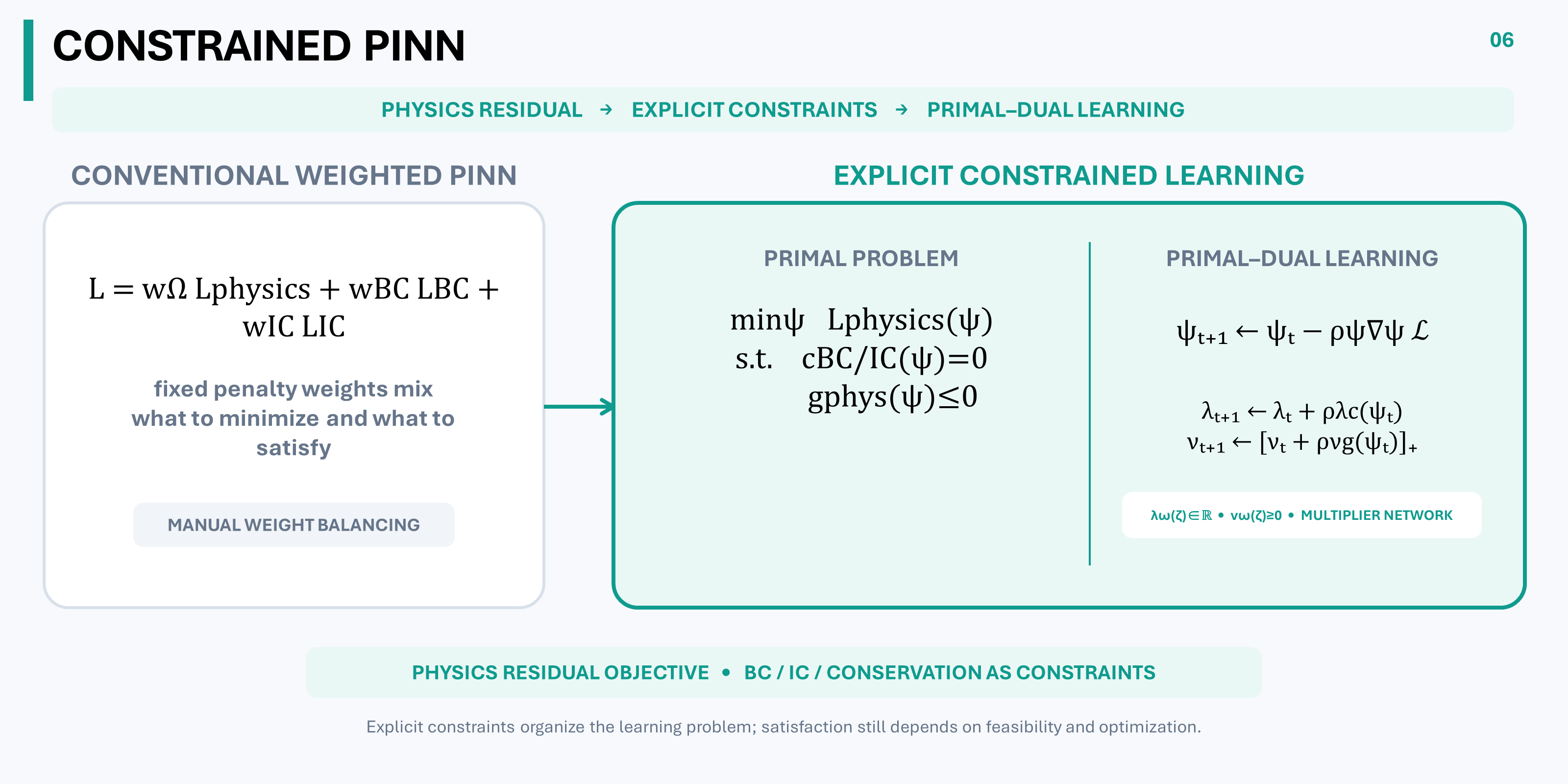
Physics and data define an explicit constrained learning problem
whose primal and dual variables produce a physics-consistent field or model
The formulation distinguishes sampled residual minimization from continuous-domain constraint satisfaction. Writing an explicit constraint does not by itself establish feasibility or convergence.
1. Problem definition
This Theme concerns the model and state-information side of Online Learning-Based Optimal Control, but PINNs also apply well beyond control. It therefore begins from the general problem of learning a physical field or model rather than from a Bellman decision problem.
Within the MIC Lab program, Constrained PINN is primarily a supporting physics-learning capability: it can prepare or update a control-usable model or state representation for an online estimator, predictor, critic target, or controller.
Let $q$ denote the physical field or model and let $\widehat q_\psi(\zeta)$ be its primal neural approximation, parameterized by $\psi$. The coordinate $\zeta$ may contain space, time, geometry, material parameters, and operating conditions. For a governing operator $\mathcal N$, define the interior physics residual
\[r_\Omega(\zeta;\psi) = \mathcal N \!\left( \widehat q_\psi \right)(\zeta) - b(\zeta),\]where $b(\zeta)$ is the declared source or forcing term. Let $\mathcal C_\Omega$ be the interior collocation set; the corresponding loss is
\[\mathcal L_{\mathrm{physics}}(\psi) = \frac{1}{|\mathcal C_\Omega|} \sum_{\zeta\in\mathcal C_\Omega} \left\| r_\Omega(\zeta;\psi) \right\|^2.\]For a forward problem, set $\mathcal L_{\mathrm{obj}}=\mathcal L_{\mathrm{physics}}$. For an inverse problem or sparse-data reconstruction, an observation term may be included:
\[\mathcal L_{\mathrm{obj}}(\psi) = \mathcal L_{\mathrm{physics}}(\psi) + w_{\mathrm{obs}}\mathcal L_{\mathrm{obs}}(\psi), \qquad w_{\mathrm{obs}}\ge0.\]The observation term remains part of the objective rather than one of the declared physical constraints. Here $\mathcal L_{\mathrm{obs}}$ denotes the observation-data misfit.
Boundary, initial, conservation, interface, and admissibility conditions are represented as equality and inequality residuals:
\[c_j(\zeta;\psi)=0 \quad \forall\zeta\in\mathcal C_j^{=}, \qquad d_m(\zeta;\psi)\le0 \quad \forall\zeta\in\mathcal C_m^{\le}.\]Here $j=1,\ldots,J$ and $m=1,\ldots,M$. Scalar residuals are shown for clarity; components of vector-valued residuals are stacked in the same way. The sets $\mathcal C_j^{=}$ and $\mathcal C_m^{\le}$ specify where sampled equality and inequality constraints are enforced.
For example,
\[\begin{aligned} c_{\mathrm{BC}}(\zeta;\psi) &= \mathcal B\!\left(\widehat q_\psi\right)(\zeta) - b_{\partial\Omega}(\zeta),\\ c_{\mathrm{IC}}(s;\psi) &= \widehat q_\psi(s,0)-q_0(s). \end{aligned}\]$\mathcal B$ is the boundary operator, $b_{\partial\Omega}$ is the prescribed boundary data, and $q_0$ is the initial field over the spatial coordinate $s$.
The defining optimization problem places the physics residual and any observation loss in the objective, and the remaining requirements after an explicit $\mathrm{s.t.}$ line:
\[\begin{aligned} \min_{\psi}\quad &\mathcal L_{\mathrm{obj}}(\psi)\\ \mathrm{s.t.}\quad &c_j(\zeta;\psi)=0 \quad \forall\zeta\in\mathcal C_j^{=},\\ &d_m(\zeta;\psi)\le0 \quad \forall\zeta\in\mathcal C_m^{\le}. \end{aligned}\]This equation defines the target learning problem, not a training algorithm. For the sampled problem, each pair $(j,\zeta)$ in an equality collocation set has an unrestricted multiplier, and each pair $(m,\zeta)$ in an inequality collocation set has a nonnegative multiplier. Stacking them gives the dual vectors $\lambda$ and $\nu$, respectively. Section 5 first gives direct vector updates and then an optional shared multiplier-network parameterization that generates these entries from $\zeta$.
2. Why this problem matters
PINNs can learn complex fields or models by combining sparse observations with governing physics. A conventional PINN usually places PDE residuals, boundary conditions, initial conditions, data, and conservation terms in one weighted sum. Large differences in scale and conditioning can cause training to reduce one term while leaving another physically important condition poorly satisfied.
An explicit constrained formulation separates what should be minimized from what should be satisfied. With appropriate residual scaling, convergence, and constraint qualifications, the associated Lagrange multipliers can provide local sensitivity information, and nonzero inequality multipliers can help identify active constraints. Raw magnitudes are not directly comparable across differently scaled residuals. This can make the learning problem more transparent and reduce manual penalty-weight tuning, but it does not automatically produce an exact physical solution or a convergent algorithm.
3. Key challenges
- Feasibility and representation: the network class, collocation set, and coupled physical conditions may not admit a feasible solution.
- Nonconvex primal–dual learning: simultaneous primal-network and dual updates can oscillate, diverge, or become poorly scaled.
- Sampled versus continuous satisfaction: small residuals at collocation points do not prove physical consistency throughout the domain or under new conditions.
- Multiplier representation and computation: independently optimized pointwise multipliers scale with the collocation set; a shared multiplier network adds approximation choices, regularization, gradient-computation cost, and another coupled learning problem.
4. Baselines — weighted penalties and hard parameterization
The standard soft-penalty PINN minimizes
\[\mathcal L_{\mathrm{pen}}(\psi) = w_\Omega \mathcal L_{\mathrm{physics}}(\psi) + w_{\mathrm{BC}} \mathcal L_{\mathrm{BC}}(\psi) + w_{\mathrm{IC}} \mathcal L_{\mathrm{IC}}(\psi) + \sum_r w_r\mathcal L_r(\psi), \qquad w_\Omega,w_{\mathrm{BC}},w_{\mathrm{IC}},w_r\ge0.\]$\mathcal L_{\mathrm{BC}}$ and $\mathcal L_{\mathrm{IC}}$ are the sampled boundary- and initial-residual losses, while $r$ indexes any additional residual penalties.
Fixed weights are simple, and adaptive loss balancing can reduce some scale mismatch. Nevertheless, a finite penalty permits constraint violation, whereas a very large penalty can make optimization ill-conditioned.
For a selected simple equality condition, a separate hard baseline is
\[\widehat q_\psi(\zeta) = q_{\mathrm{known}}(\zeta) + A(\zeta)h_\psi(\zeta)\]This parameterization is chosen before training, rather than applied as a correction afterward. Here $q_{\mathrm{known}}$ satisfies the prescribed condition, $h_\psi$ is an unconstrained neural correction, and $A(\zeta)$ is zero wherever that value condition must hold. For example, the initial condition $q(s,0)=q_0(s)$ can be encoded as
\[\widehat q_\psi(s,\tau) = q_0(s)+\tau h_\psi(s,\tau).\]At physical time $\tau=0$, the neural correction vanishes for every $\psi$, so the initial condition remains exactly satisfied throughout training. For a derivative or operator constraint, $A=0$ alone is insufficient: the parameterization must make the relevant operator applied to the correction vanish. Hard encoding is therefore useful for selected simple equalities but can be difficult to construct for complex geometries, coupled interfaces, inequalities, or changing conditions.
5. Research direction — explicit constraints and primal–dual learning
At the sampled level, stack equality and inequality residuals over their collocation sets as $c(\psi)$ and $d(\psi)$. The Lagrangian is
\[\mathscr L(\psi,\lambda,\nu) = \mathcal L_{\mathrm{obj}}(\psi) + \lambda^\top c(\psi) + \nu^\top d(\psi), \qquad \nu\ge0.\]At primal–dual training iteration $t$, distinct from the physical coordinate $\tau$ used above, conceptual updates are
\[\begin{aligned} \psi_{t+1} &= \psi_t - \rho_{\psi,t} \nabla_\psi \mathscr L(\psi_t,\lambda_t,\nu_t),\\ \lambda_{t+1} &= \lambda_t + \rho_{\lambda,t}c(\psi_t),\\ \nu_{t+1} &= \left[ \nu_t + \rho_{\nu,t}d(\psi_t) \right]_+ . \end{aligned}\]Here $\rho_{\psi,t},\rho_{\lambda,t},\rho_{\nu,t}>0$, and $[\cdot]_+$ denotes componentwise projection onto the nonnegative orthant. Equality multipliers $\lambda$ are unrestricted, so their update is signed. The projected inequality update increases a multiplier for positive violation and can decrease it when the corresponding constraint is strictly satisfied. The primal step updates the learned field or model. Augmented-Lagrangian terms, residual normalization, alternating updates, and dual regularization are possible stabilization mechanisms rather than guarantees.
The updates above optimize one multiplier entry per sampled residual. Shared multiplier networks can instead generate domain-indexed entries:
\[\lambda_j(\zeta) = \Lambda_{\omega_\lambda,j}(\zeta), \qquad \nu_m(\zeta) = \operatorname{softplus} \!\left( R_{\omega_\nu,m}(\zeta) \right) \ge0.\]$\Lambda_{\omega_\lambda,j}$ is the equality-network output, and $R_{\omega_\nu,m}$ is the raw inequality-network output, with $\omega_\lambda$ and $\omega_\nu$ denoting their parameters. The equality multiplier needs no sign transformation, while softplus enforces $\nu_m\ge0$. At each collocation batch, these outputs supply $\lambda$ and $\nu$ in the sampled Lagrangian; $\psi$ is updated by descent and the multiplier-network parameters by dual ascent. This shares a parameterization across points but restricts the dual class, so sampled feasibility still does not establish continuous-domain feasibility.
Future evidence should compare a baseline PINN, fixed and adaptive penalties, hard encoding where available, directly optimized multiplier vectors with standard or augmented-Lagrangian updates, and a multiplier-network variant under matched data and computation budgets. Metrics should include reference-solution error, physics residual, mean and maximum constraint violation, conservation defect, training stability, multiplier behavior, computation, and generalization to new boundary conditions, parameters, and geometries.
6. Application domains
- Structural, contact, and multiphysics systems, where interface, conservation, positivity, or material conditions must be distinguished from the governing residual objective.
- Sparse-observation inverse problems and state reconstruction, where physical constraints supplement incomplete measurements.
- Synchronous-machine flux-linkage learning and estimation, where governing electrical dynamics and physically admissible inductance bounds guide online learning of a nonlinear magnetic model. A related MIC Lab study reports simulation validation on a 35-kW IPMSM drive (Jang, Ryu, and Choi, 2025).
- EV battery and thermal-management analysis, including temperature-field reconstruction under changing cooling conditions and sparse sensing.
References
- S. Jang, M. Ryu, and K. Choi, “Physics-Informed Online Learning of Flux Linkage Model for Synchronous Machines,” IECON 2025 — 51st Annual Conference of the IEEE Industrial Electronics Society, pp. 1–6, 2025. IEEE Xplore · Full text