Mobility-System-Level Optimal Control
Core idea. Mobility-system-level optimal control uses information and decision couplings beyond the local vehicle boundary. It includes both a single vehicle using traffic-network context for long-horizon operation and multiple vehicles coordinating through shared information.
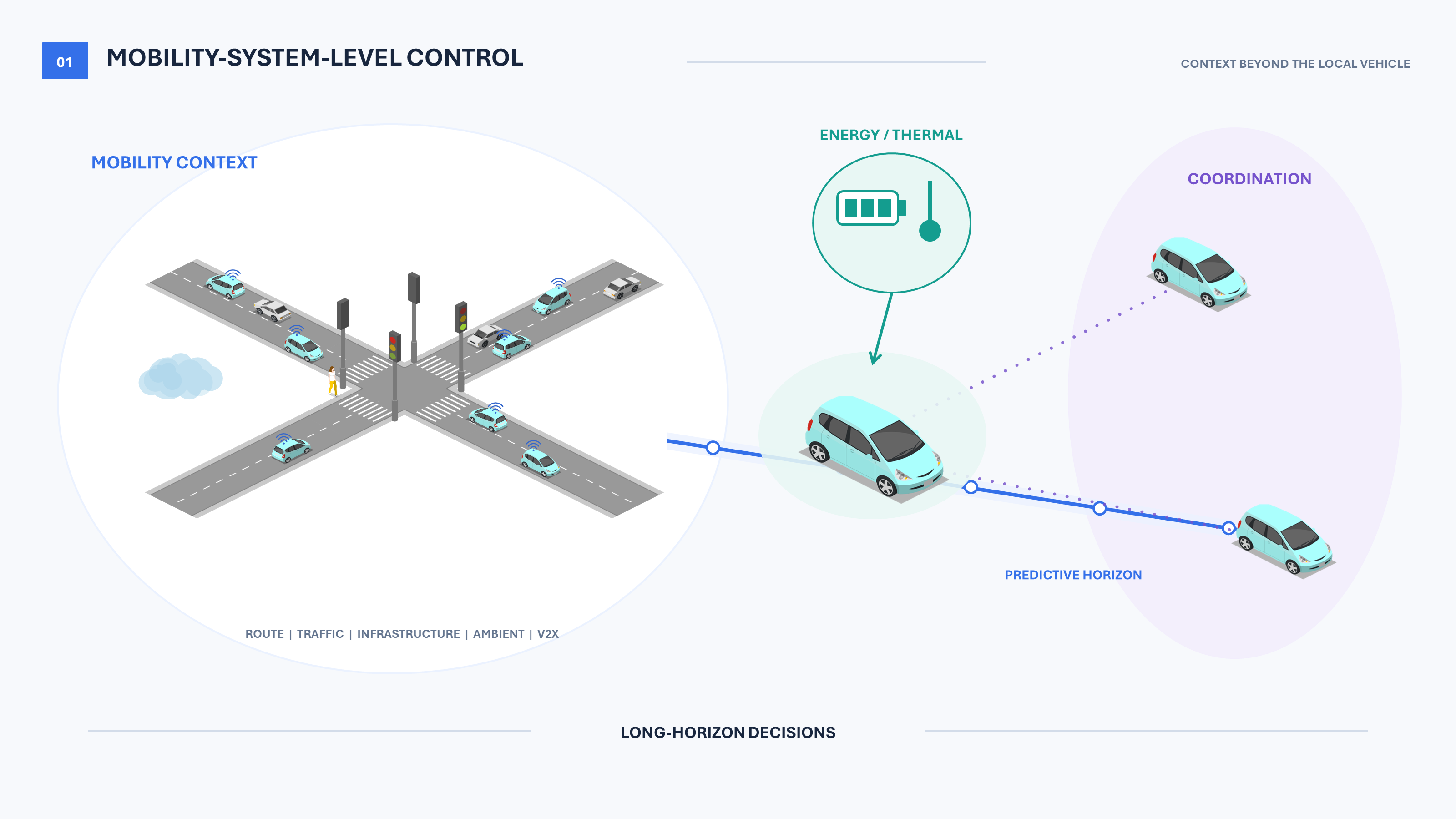
Route, traffic, infrastructure, ambient, and vehicle-to-everything (V2X) information
form a mobility-system decision state for energy, thermal, and coordination control.
The number of controlled vehicles does not define the level by itself. The defining feature is the information and decision scope used by the controller.
1. Scope: control beyond the local vehicle boundary
Future Mobility Control Landscape defines mobility-system-level control by an information or decision scope that extends beyond the local vehicle boundary. In addition to onboard measurements, a controller may use road grade, signal phase and timing, traffic flow, route or mission information, weather and ambient conditions, charging or refueling availability, and vehicle-to-everything (V2X) messages from vehicles or infrastructure. The relevant agents can include connected and automated vehicles, human-driven vehicles, infrastructure, fleets, and shared energy resources.
This broader information enables a wider set of coupled decisions: current and future power or thermal allocation, speed and trajectory planning, route and charging choices, and coordination among vehicles. It also enlarges the prediction horizon, state and action spaces, and set of interaction and resource constraints. The control problem becomes mobility-system-level when these external information sources, cross-agent coupling, or long-run consequences across repeated trips materially change the objective, dynamics, or constraints.
Energy and thermal management illustrate the boundary. They are mobility-system-level when route, traffic, infrastructure, ambient forecasts, or long-run network operation determine the decision. The same actuators can form a vehicle-level problem when the controller uses only onboard states and the current local power or thermal demand.
2. Representative control problems
| Problem | Representative decisions | Objectives | Main constraints |
|---|---|---|---|
| Electrified-vehicle (xEV) predictive energy and/or thermal management | power-source allocation, battery use, cooling or heating, charging or refueling decisions | energy or fuel use, thermal performance, degradation, and long-run reserve | power balance, state of charge, temperatures, actuator limits, and route feasibility |
| Multi-vehicle coordination | speed, spacing, trajectory, merging, or shared-resource decisions | safety, throughput, travel time, energy, and comfort | collision avoidance, road geometry, actuator limits, communication, and distributed information |
Multi-vehicle coordination is mobility-system-level because vehicle decisions are coupled through safety, traffic flow, or shared resources. It is distinct from single-vehicle predictive energy and thermal management and is not required for every mobility-system-level problem.
3. xEV predictive energy management
Suppose an xEV has an intended trip or predicted driving segment covering physical sampling steps $k=0,\ldots,T$. Let $x_k$ collect its energy states, $u_k$ denote power-source allocation, and $w_k$ contain predicted route-dependent traction and auxiliary demand. A generic predictive energy-management problem is
\[\begin{aligned} \min_{u_0,\ldots,u_{T-1}}\quad& \sum_{k=0}^{T-1} g_{\mathrm E}(x_k,u_k,w_k) + \Phi_T(x_T)\\ \mathrm{s.t.}\quad& x_{k+1}=f(x_k,u_k,w_k),\\ & (x_k,u_k)\in\mathcal Z_k,\qquad x_T\in\mathcal X_T . \end{aligned}\]$g_{\mathrm E}$ represents fuel or electrical-energy use and possibly degradation; $\Phi_T$ and $\mathcal X_T$ describe the terminal energy requirement. Power balance, source and battery limits, and state-of-charge constraints are included in $f$ and $\mathcal Z_k$.
A fuel-cell electric vehicle (FCEV) is one concrete instance: $x_k$ can be battery state of charge (SOC), $u_k$ fuel-cell power, and, for sampling interval $\Delta t$, let $g_{\mathrm E}(x_k,u_k,w_k)=\Delta t\,\dot m_{\mathrm{fc}}(u_k)$ denote the hydrogen consumed over one step. Equivalently, $\Delta t$ may be absorbed into the stage-cost definition. The battery supplies the residual traction demand through the power balance. When the mission requires a prescribed terminal energy state, it can be imposed through the hard terminal set $\mathcal X_T={x_{\mathrm{tar}}}$.
The physical model need not be written as $f_k$. A time-varying preview $w_k$ induces the effective dynamics and cost
\[F_k(x,u):=f(x,u,w_k), \qquad G_k(x,u):=g_{\mathrm E}(x,u,w_k),\]so the problem is nonstationary in physical time when represented by $x$ alone, even if the underlying plant function $f$ is time invariant. This time dependence does not by itself imply uncertainty: the problem is nonstationary even when the complete sequence ${w_k}$ is known. Uncertainty arises because future power demand, traffic, route, and ambient context are usually predicted imperfectly.
If the mission truly ends at $T$, the finite-horizon formulation can define the correct optimal-control problem. For a vehicle operating continuously across trips, however, the performance horizon is effectively infinite. A finite trip or prediction horizon is then only an approximation and requires a terminal value that represents consequences beyond $T$.
4. Coupled predictive extensions
Multi-vehicle coordination within the predictable horizon
The full multi-vehicle coordination domain includes safety, traffic flow, and shared-resource objectives beyond energy management. The following formulation is one coupled example in which coordination forms the short-horizon part of predictive energy and thermal management. Let $Z_k$ collect the joint vehicle and traffic states, $U_k$ the speed, trajectory, or coordination decisions, $S_k$ the vehicles’ energy and thermal states, and $V_k$ their energy and thermal controls. The coordination decisions determine the predicted traction and thermal demands:
\[w_{j\mid k}^i = \mathcal D^i \!\left(Z_{j\mid k},U_{j\mid k}\right), \qquad i=1,\ldots,N_{\mathrm{veh}} .\]Here $j\mid k$ denotes a $j$-step-ahead prediction made at decision time $k$, $H$ is the prediction horizon, $N_{\mathrm{veh}}$ is the number of vehicles, and $\mathcal D^i$ maps the joint motion prediction to vehicle $i$’s demand. Let $w_{j\mid k}$ collect these per-vehicle predicted demands. The symbols $U$ and $V$ below denote the corresponding decision sequences over the horizon.
A coupled short-horizon problem can then be written as
\[\begin{aligned} \min_{U,V}\quad& \sum_{j=0}^{H-1} \alpha^j \Big[ g_{\mathrm{coord}}(Z_{j\mid k},U_{j\mid k}) + g_{\mathrm{E/T}}(S_{j\mid k},V_{j\mid k},w_{j\mid k}) \Big] + \alpha^H J_{\mathrm{long}}(S_{H\mid k},Z_{H\mid k})\\ \mathrm{s.t.}\quad& \text{vehicle and energy--thermal dynamics,}\\ & \text{road, collision, actuator, and information constraints.} \end{aligned}\]Here $g_{\mathrm{coord}}$ and $g_{\mathrm{E/T}}$ are the coordination and aggregate per-vehicle energy–thermal stage costs, $J_{\mathrm{long}}$ is the beyond-horizon value, and $0<\alpha\le 1$ is the finite-horizon discount factor. Its argument $Z_{H\mid k}$ supplies the mobility context needed to evaluate long-run consequences beyond the energy and thermal state $S_{H\mid k}$.
The explicit horizon uses predictable traffic interactions to optimize coordination, energy, and thermal performance while enforcing immediate safety and physical constraints. The terminal value $J_{\mathrm{long}}$ evaluates energy and thermal consequences beyond the reliable prediction horizon. Thus, coordination changes the near-term demand trajectory, whereas the terminal cost supplies the longer-run perspective.
Coupled energy–thermal extension
Thermal management has an analogous structure after augmenting the energy state and control. For example,
\[s_k= \begin{bmatrix} x_k & T_{\mathrm{bat},k} & T_{\mathrm{fc},k} \end{bmatrix}^{\!\top}, \qquad v_k= \begin{bmatrix} u_k & P_{\mathrm{pump},k} & P_{\mathrm{fan},k} \end{bmatrix}^{\!\top}.\]Here $x_k$ is the energy state introduced in Section 3, such as battery SOC; $T_{\mathrm{bat},k}$ and $T_{\mathrm{fc},k}$ are the battery and fuel-cell temperatures; and $u_k$ is the power-source allocation. The variables $P_{\mathrm{pump},k}$ and $P_{\mathrm{fan},k}$ are the commanded electrical powers of the coolant pump and radiator fan. Thus, $T_{\cdot,k}$ denotes temperature, whereas $H$ below is the prediction-horizon length. Let $w_k$ collect the predicted traction demand and thermal context, including ambient conditions.
A representative problem is
\[\begin{aligned} \min_{v_0,\ldots,v_{H-1}}\quad& \sum_{k=0}^{H-1} \left[ \ell_{\mathrm{energy}}(s_k,v_k,w_k) + \rho_{\mathrm{th}}\ell_{\mathrm{thermal}}(s_k) \right] + J_{\mathrm{E/T}}^{\mathrm{tail}}(s_H)\\ \mathrm{s.t.}\quad& s_0=s_{\mathrm{init}},\\ & s_{k+1}=F_k^{\mathrm{E/T}}(s_k,v_k,w_k), \qquad k=0,\ldots,H-1,\\ & \underline s_k\le s_k\le\overline s_k, \qquad k=0,\ldots,H,\\ & \underline v_k\le v_k\le\overline v_k, \qquad k=0,\ldots,H-1 . \end{aligned}\]Here $\ell_{\mathrm{energy}}$ accounts for fuel or electrical-energy use and, when relevant, degradation; $\ell_{\mathrm{thermal}}$ penalizes undesirable temperature operation; and $\rho_{\mathrm{th}}\ge 0$ sets their relative weight. $J_{\mathrm{E/T}}^{\mathrm{tail}}$ evaluates energy and thermal consequences beyond the prediction horizon. $s_{\mathrm{init}}$ is the measured or estimated initial augmented state, $F_k^{\mathrm{E/T}}$ is the context-dependent coupled energy–thermal transition map, and the underlined and overlined quantities are the state and control bounds.
The problem is mobility-system-level when route, traffic, charging, or ambient forecasts materially determine these decisions; with only local states and demand, the same formulation is vehicle-level.
5. Why these predictive problems are difficult
-
Information and formulation limitations: future traction-power demand $w_k$, route, traffic, ambient conditions, and other agents evolve with physical time and location. Consequently, the dynamics, cost, constraints, or disturbance distribution can be time- or context-dependent. One stationary policy or value function (critic) need not represent the exact optimum unless sufficient context is included or the problem is reformulated. An approximate or robust stationary policy may still be useful under stated conditions. Missing transition and context models, prediction uncertainty, and estimation of SOC or temperature also limit the information available to the controller.
-
Computational difficulty: long horizons, nonlinear battery, fuel-cell, and thermal dynamics, hybrid operating modes, coupled vehicle or resource decisions, and numerous state, actuator, safety, and collision constraints produce large optimization or dynamic-programming problems. The solution must still be updated within the relevant online control deadline.
The information and formulation barrier determines which representation, prediction, estimation, or reformulation is needed to define the decision problem; computational difficulty limits how accurately it can be solved online.
6. Two research questions
The application problems above lead to two research questions:
- How can a time- and context-dependent mobility-system problem be converted into a reusable long-run optimal-control problem despite uncertain future context?
- How can its value and current decisions be computed or approximated within an online deadline, especially for nonlinear energy–thermal systems or coupled multi-vehicle decisions?
7. MIC Lab approach and connections to research themes
The xEV formulation is one concrete MIC Lab pathway. The cited hybrid electric vehicle (HEV) and FCEV studies document successive steps in that pathway; they do not prescribe how every mobility-system problem must be solved.
7.1 Nonstationarity and context uncertainty: construct a reusable long-run critic
Nonstationary Infinite-Horizon OCP addresses the first research question. In this application, the physical-time problem is first aggregated over road links so that repeated operation can be represented by a reusable network state rather than by absolute physical time.
Let $k$ denote a physical sampling step, $n$ a link step, $q_n$ the current road link, $\bar x_n$ the energy state at the entry boundary of $q_n$, and $a_n$ a link-level decision parameter. The time-domain dynamics, costs, and preview within link $q_n$ are reduced to a link-domain transition and cost:
\[\left\{ F_k,\ G_k,\ w_k \right\}_{k\ \mathrm{within}\ q_n} \quad\longrightarrow\quad \begin{cases} \bar x_{n+1}=F_{q_n}(\bar x_n,a_n),\\ \ell_{q_n}(\bar x_n,a_n). \end{cases}\]The 2024 T-ITS study provides the within-route reduction: time-sampled demand over a known finite route is summarized by link-level energy and duration information, while the route horizon and terminal energy requirement remain explicit. The 2026 study extends the same link-domain foundation to repeated operation over a traffic network. It adds stochastic transitions among links and treats $(\bar x_n,q_n)$ as a persistent network state.
If $p_{qq’}=\Pr(q_{n+1}=q’\mid q_n=q)$ is the link-transition probability, the reusable network value satisfies
\[J_{\mathrm{net}}^\star(\bar x,q) := \min_{a\in\mathcal A(\bar x,q)} \left\{ \ell_q(\bar x,a) + \gamma \sum_{q'}p_{qq'} J_{\mathrm{net}}^\star \!\left(F_q(\bar x,a),q'\right) \right\}.\]Here $\mathcal A(\bar x,q)$ is the admissible set of link-level decisions, $F_q$ and $\ell_q$ are the aggregated transition and cost, and $0<\gamma<1$ is the long-run discount factor. Value iteration computes this long-run value function, or critic, from the link-level model and transition statistics. During operation, its expected terminal value is appended to the finite predicted-link problem. The optimizer can then select the terminal energy state by balancing the current route against subsequent network operation, rather than imposing a fixed terminal-energy target.
7.2 Computational difficulty: approximate DP and online multistep lookahead
When the state or context space is too large for tabular value iteration, Online Learning-Based Optimal Control uses approximate dynamic programming (ADP) to represent the long-run value or policy. Let $\zeta=(\bar x,q)$ denote the link-domain state and $\theta$ the critic parameters; then
\[\widehat J_{\theta}(\zeta) \approx J_{\mathrm{net}}^\star(\bar x,q).\]For the current prediction, Online Multistep Lookahead holds this critic fixed. More generally, let $\zeta_{j\mid k}$ denote the predicted application state, $a_{j\mid k}$ its decision, $A_k=(a_{0\mid k},\ldots,a_{H-1\mid k})$ the decision sequence, and $g_{\mathrm{use}}$ the declared stage cost. The online problem has the form
\[\widehat A_k^{(H)} \in \arg\min_{A_k} \left\{ \sum_{j=0}^{H-1} \alpha^j g_{\mathrm{use}}(\zeta_{j\mid k},a_{j\mid k}) + \alpha^H \widehat J_{\theta}(\zeta_{H\mid k}) \right\}.\]For link-domain energy management, $\zeta=(\bar x,q)$ and $a$ is a link decision. For the coupled formulation in Section 4, $\zeta$ collects $(S,Z)$ and $a$ collects $(V,U)$. The resulting multistep solution can be executed directly or used to train a policy network online. The 2026 FCEV study uses link-based tabular value iteration and direct finite-horizon optimization; critic approximation and online policy training are broader research extensions.
7.3 Additional learning-based connections
Other themes can support different missing pieces:
| Research theme | Possible role in this control domain |
|---|---|
| Continual Model Learning | Update power-demand, traffic-transition, degradation, or thermal models while retaining behavior learned in earlier operating regions. |
| Structured Critic Adaptation | Reconfigure a prelearned long-run critic using identified traffic, demand, weather, or degradation parameters. |
| Semantic Critic Learning | Incorporate incident, map, rule, mission, or scene semantics that are not captured by a compact numerical network state. |
| Real-World RL | Learn critic and policy from real streaming operation when simulation or explicit network models omit important effects. |
8. References
- K. Choi, G. Park, and D. Kum, “An Analytical Approach to the Predictive Energy Management of Connected HEVs: What Information Do We Need to Guarantee Global Optimality?,” IEEE Transactions on Intelligent Transportation Systems, vol. 25, no. 9, pp. 12749–12761, 2024.
- K. Choi, “Traffic Network-Aware Energy Management for FCEVs: Integrating Trip-Specific Control and Long-Run Optimality,” Asian Control Conference, 2026. [Full text]