Component-Level Optimal Control
Core idea. Component-level optimal control converts a torque command into fast voltage or inverter-switching decisions while minimizing drive loss or another performance index and satisfying current and voltage limits. Automatic calibration is a coupled deployment workflow that seeks to reproduce this behavior across the real electric drive’s operating domain under declared verification checks.
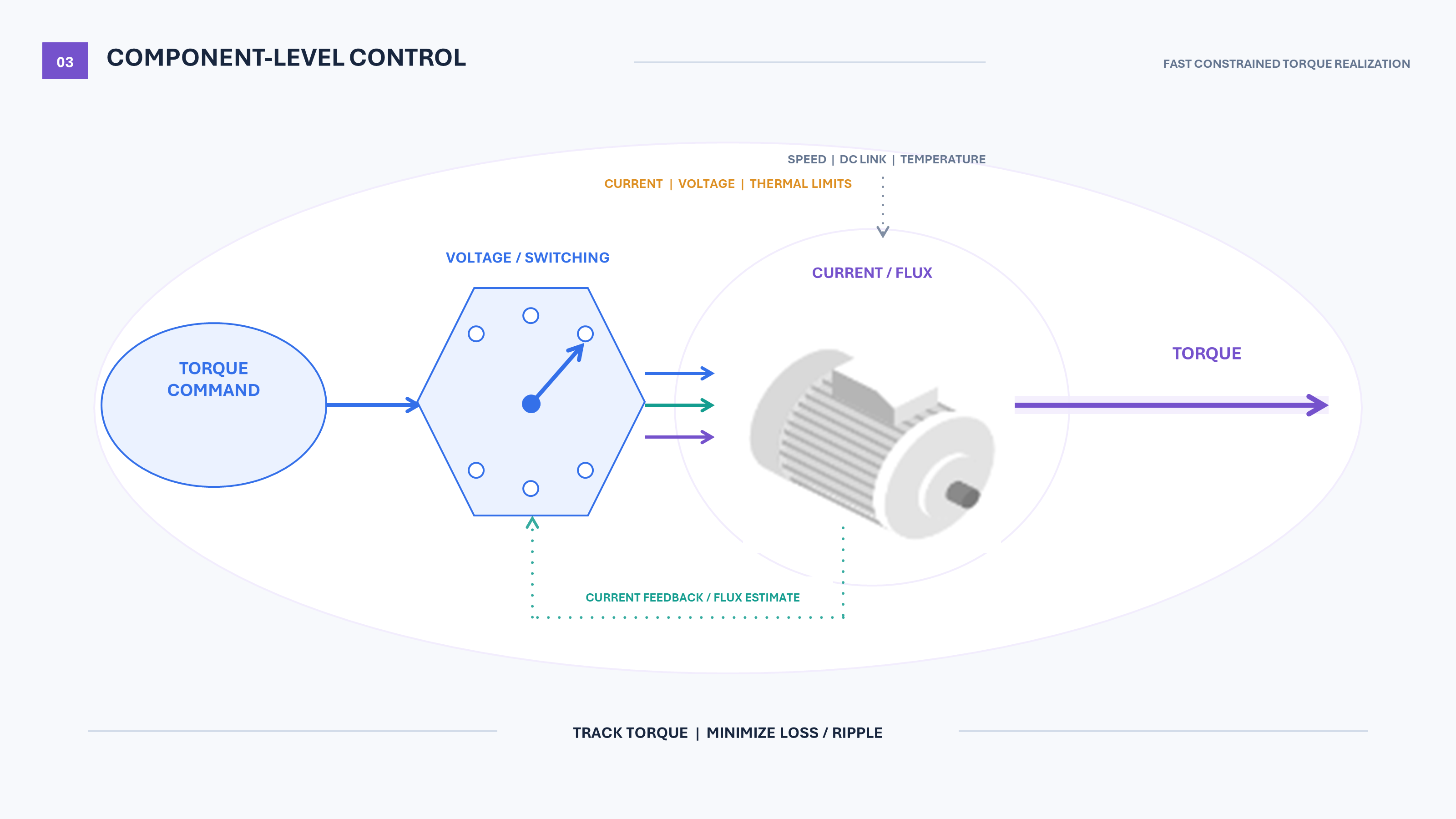
A torque command is converted into constrained voltage or inverter-switching actions
that shape current and flux to produce torque.
The component-level controller realizes the requested torque through fast electrical actuation, while current feedback and flux estimation support the drive-level loop.
1. Scope: optimal control at the electric-drive component
Future Mobility Control Landscape defines component-level control first by a device-level performance objective and coupled decision boundary. The physical-device timescale is a secondary descriptor. For an electric drive, the representative component is a synchronous machine and its inverter. The controller acts on electrical variables much faster than vehicle or mobility-system controllers act on motion, energy, or traffic decisions.
Representative elements are
| Role | Examples |
|---|---|
| Commands and context | torque command, rotor speed or position, DC-link voltage, machine temperature, and operating mode |
| Decision state | direct–quadrature ($dq$) stator current, stator flux linkage, inverter state, and selected thermal or loss-related states |
| Control inputs | continuous stator-voltage command or discrete inverter switching action |
| Performance | torque tracking, copper/iron/inverter loss, torque and current ripple, switching behavior, and transient response |
| Constraints | current, voltage, inverter switching, thermal, sampling-time, and actuator-feasibility limits |
Torque is the mechanical interface between the electric drive and the system it actuates. Rotor speed and position evolve through the balance between electromagnetic torque and the mechanical load, and propulsion, steering, robotic, and industrial systems are driven through this torque. Accurately producing a requested torque while using the available electrical degrees of freedom efficiently is therefore a central component-level control problem.
The boundary is determined by the objective. A higher-level vehicle or motion controller may decide the required wheel or shaft torque; the component-level controller realizes that command by choosing voltage or inverter-switching inputs that shape the resulting current and flux trajectories. If the primary objective instead coordinates several vehicle actuators or trip-scale energy, the problem moves to the vehicle or mobility-system level even though an electric motor executes the final action.
This page uses synchronous-machine torque control as the representative problem. The same control logic—fast constrained actuation under uncertain device physics—can extend to other electric drives and mechatronic components.
2. Representative control problem and deployment workflow
| Role | Main decisions | Main objective |
|---|---|---|
| Physical control problem — Optimal torque control | choose voltage or inverter switching actions to shape the resulting current/flux trajectory | track the commanded torque while minimizing drive loss, ripple, switching, or another performance index under current and voltage limits |
| Cross-cutting deployment workflow — Automatic calibration of electric-drive controllers | select and adjust current-, torque-, speed-, position-, estimator-, and solver-related parameters | reproduce the intended tracking, efficiency, robustness, and constraint behavior across speed, torque, temperature, DC-link, load, and machine conditions |
These are two coupled stages in the controller deployment workflow, not two physical control levels. Optimal torque control determines the electrical action for a fixed model, controller structure, and calibration. Automatic calibration then adjusts gains, maps, loss weights, observer parameters, limits, filters, and numerical-solver parameters so that the measured hardware response satisfies the intended performance and feasibility objectives throughout the declared operating domain.
The calibration problem can include the surrounding drive loops. A torque or current controller is usually embedded inside speed and position loops, while state or parameter estimators supply quantities not measured directly. Calibrating each block independently may not reproduce the desired behavior of the complete interconnected drive.
3. Optimal torque control and its calibration workflow
3.1 Optimal torque control
Let $x_k$ collect the controller-relevant electrical and inverter state, $u_k$ denote a continuous voltage vector or discrete switching action, $T_{e,k}$ the electromagnetic torque, and $\eta_k$ the control-relevant operating condition. A control-usable model has the form
\[\begin{aligned} x_{k+1} &= f \!\left( x_k, u_k; \eta_k \right),\\ T_{e,k} &= \mathcal T \!\left( x_k; \eta_k \right),\\ y_k &= h(x_k)+\nu_k . \end{aligned}\]Here $y_k$ is the measured output, $h$ the measurement map, and $\nu_k$ the measurement disturbance. $\eta_k$ may contain rotor speed, DC-link voltage, temperature, resistance, or magnetic-model information. In particular, nonlinear stator flux linkage is a function of current and operating condition:
\[\boldsymbol\lambda_{dq,k} = \Lambda \!\left( \boldsymbol i_{dq,k}; \eta_k \right).\]Depending on the chosen machine representation, $\boldsymbol\lambda_{dq,k}$ can be included explicitly in $x_k$ or reconstructed from current and operating condition through a known or learned map $\Lambda$. The latter case makes flux-model learning and flux estimation part of the information needed for torque control.
At physical time $k$, a representative finite-horizon predictive torque-control problem with horizon $H<\infty$ is written over $U_k=(u_{0\mid k},\ldots,u_{H-1\mid k})$:
\[\begin{aligned} U_k^\star \in \arg\min_{U_k}\quad& \sum_{j=0}^{H-1} \alpha^j \Big[ q_T \left\| T_{e,j+1\mid k}-T_{j+1\mid k}^{\mathrm{cmd}} \right\|^2 + \ell_{\mathrm{perf}} \!\left( x_{j+1\mid k}, u_{j\mid k} \right) \Big]\\ &+ \alpha^H V_{\mathrm f}(x_{H\mid k})\\ \mathrm{s.t.}\quad& x_{0\mid k} = \widehat x_k,\\ & x_{j+1\mid k} = f_{\mathrm{use}} \!\left( x_{j\mid k}, u_{j\mid k}; \widehat\eta_k \right), \quad j=0,\ldots,H-1,\\ & \left\| \boldsymbol i_{dq,j+1\mid k} \right\| \le I_{\max}, \quad j=0,\ldots,H-1,\\ & u_{j\mid k} \in \mathcal U_{\mathrm{inv}}, \quad j=0,\ldots,H-1. \end{aligned}\]$T_{j+1\mid k}^{\mathrm{cmd}}$ is the predicted torque command, $q_T\ge0$ its tracking weight, and $0<\alpha\le1$ the finite-horizon discount factor. The vectors $\boldsymbol i_{dq}$ and $\boldsymbol v_{dq}$ are the $dq$ current and voltage, and $I_{\max}$ is the allowable current magnitude. $f_{\mathrm{use}}$ is the declared known or learned prediction model. $V_{\mathrm f}$ is the finite-horizon terminal value, possibly supplied by a learned value-function approximation (critic). $\ell_{\mathrm{perf}}$ can represent copper, iron, or inverter loss, switching activity, ripple, thermal stress, or another declared drive-level objective. For a two-level voltage-source inverter, $\mathcal U_{\mathrm{inv}}$ is the DC-link-dependent voltage hexagon in a continuous-input implementation or the finite set of admissible inverter voltage vectors in direct finite-control-set switching.
The Generalized Model Predictive Torque Control (GMPTC) study provides a concrete one-step instance. It enforces torque, current, and voltage feasibility while allowing a declared combination of copper, iron, and inverter loss. When the requested torque is infeasible, it instead maximizes achievable torque in the commanded direction. GMPTC supports continuous or finite inverter control sets and is a practical constrained short-horizon realization, not an infinite-horizon solution.
The preceding problems are finite-horizon formulations: GMPTC uses $H=1$, while a longer-horizon model predictive controller (MPC) uses a finite $H>1$. Receding-horizon execution may continue indefinitely, but each online optimization explicitly evaluates only the next $H$ stages and represents everything beyond them through $V_{\mathrm f}$. If that terminal value does not accurately represent the long-run consequence, near-term torque and loss optimization can remain suboptimal over continuous operation.
The ideal long-run decision problem can instead be defined directly as an infinite-horizon optimal-control problem (OCP). For this definition, $x_k$ is understood to be augmented with the torque command, rotor speed, DC-link condition, temperature, and any other context required to make the decision state Markov. This augmentation is valid only when the context dynamics or transition law and the probability law underlying the expectation are also specified:
\[\mu^\star \in \arg\min_{\mu} \mathbb E \left[ \sum_{j=0}^{\infty} \alpha^j g \!\left( x_{k+j}, \mu(x_{k+j}) \right) \right], \qquad 0<\alpha<1,\]subject to the electric-drive dynamics and current, voltage, thermal, and switching constraints, where $g$ is the declared long-run stage cost. Solving this problem would minimize the declared long-run cost directly. Because its exact solution is generally impractical, the research objective is to approximate its optimal value and policy through approximate dynamic programming (ADP). Finite-horizon MPC remains a useful online implementation, especially when $V_{\mathrm f}$ is supplied by an approximate infinite-horizon critic rather than by an arbitrary short-horizon terminal penalty.
3.2 Automatic calibration during implementation and validation
Automatic calibration is not limited to the fast torque controller. A deployed electric-drive control system can contain current or torque control, outer speed and position loops, flux and rotor-state estimators, inverter logic, and the driven mechanical plant. Their gains, maps, filters, limits, objective weights, and solver settings interact through the complete cascaded, multi-rate closed loop.
Let $r_k$ denote the command presented to this stack—such as a torque, speed, or position command—and let $\mu_\rho$ denote the resulting composite controller:
\[u_k = \mu_\rho \!\left( \widehat x_k, r_k \right).\]Here, $\widehat x_k$ contains the available electrical, mechanical, estimated, and operating-context variables. The deployable calibration vector $\rho$ collects parameters across the inner and outer controllers, estimators, constraint handling, filters, and numerical solver. Calibration can therefore evaluate the complete response from $r_k$ to torque, speed, or position rather than assuming that every inner loop is ideal.
Model-based design supplies an initial controller and calibration $\rho_0$. After implementation on the drive electronic control unit (ECU), repeated simulation, dynamometer, or system tests evaluate tracking, loss, ripple, constraint activity, robustness, and execution time:
\[\text{model-based design} \rightarrow \text{ECU/inverter implementation} \rightarrow \text{drive or system test} \rightarrow \text{evaluation} \rightarrow \text{manual recalibration}.\]Let $n$ index an accepted calibration trial, $\chi_n$ its machine, load, and operating context, $\tau_n(\rho_n)$ the measured trajectory of the complete cascaded closed loop, and $m_n$ the resulting performance and feasibility metrics. Define
\[d_n^{\mathrm{cal}} := \left( \chi_n,\rho_n,\tau_n,m_n \right), \qquad \mathcal D_{0:n}^{\mathrm{cal}} := \left\{ d_i^{\mathrm{cal}} \right\}_{i=0}^{n}.\]A data-driven tuning step can select the next admissible calibration through
\[\rho_{n+1} \in \arg\min_{\rho\in\mathcal P_n^{\mathrm{adm}}} \widehat{\mathcal L}_{\mathrm{cal},n} \!\left( \rho;\mathcal D_{0:n}^{\mathrm{cal}} \right).\]$\widehat{\mathcal L}_{\mathrm{cal},n}$ estimates the calibration objective over the declared speed, torque, temperature, DC-link, load, and machine domain. $\mathcal P_n^{\mathrm{adm}}$ is the candidate set admitted by parameter bounds, pre-test checks, current/voltage and thermal constraints, fallback logic, and ECU timing requirements. The algorithm must learn from limited safe experiments without treating constraint violations as freely available exploration.
4. Why electric-drive optimal control and calibration are difficult
-
Information and formulation limitations: the nonlinear stator flux-linkage map is central to torque prediction and constraint handling but is not measured directly. Resistance, inverter nonlinearity, iron loss, temperature, aging, and sensorless rotor-state estimation add uncertainty. The surrounding current, torque, speed, and position loops also interact through saturation, finite bandwidth, estimators, and shared model errors, so isolated block behavior does not determine the complete closed loop. Hardware calibration data remain limited because unsafe electrical, thermal, or unstable controller parameters cannot be explored freely.
-
Computational difficulty: one-step MPC can be practical. The burden grows with longer horizons, nonlinear magnetic and loss models, constrained continuous optimization, or branching over switching actions, while electrical sampling periods remain short. Exact infinite-horizon dynamic programming and online model, critic, or policy updates must also fit within embedded memory, computation, and verification limits.
5. Three research questions
- Model and state learning: How can a physically consistent flux-linkage model and the unmeasured control state be learned online across changing electrical and thermal conditions while retaining behavior learned in earlier operating regions?
- Interconnected control and calibration: How can controller and estimator parameters across the torque/current, speed, and position loops be calibrated from the behavior of the interconnected inverter–machine–mechanical closed loop rather than through isolated ideal-loop assumptions?
- Long-run embedded optimality: How can an infinite-horizon electric-drive value or policy be approximated and improved within the drive ECU’s short control deadline while preserving current, voltage, thermal, and switching feasibility?
6. MIC Lab approach and connections to research themes
The two cited papers address complementary parts of the component-level problem. GMPTC supplies a constrained short-horizon torque-control baseline under a known magnetic model. Physics-Informed Online Learning (PIOL) addresses the type of flux-model uncertainty treated as known in GMPTC. Infinite-horizon ADP, continual retention, and automatic calibration are research extensions rather than achieved claims of those papers.
6.1 Flux-model and state uncertainty: physics-constrained online learning and continual retention
The PIOL study treats stator flux linkage as a nonlinear function of measured $dq$ currents. Applying the chain rule converts the measured electrical ordinary differential equations into current-domain partial differential constraints. The neural flux model minimizes this physics residual while explicitly bounding physically meaningful self-differential inductances. PIOL estimates the current derivative by finite differences and treats stator resistance as known. This is a concrete component-level instance of a Constrained physics-informed neural network (PINN): physics residuals define the objective, physical inequalities remain explicit constraints, and primal–dual updates learn the model parameters and constraint multipliers. The learned model can also act as an online flux-linkage estimator.
PIOL demonstrated simulation-level feasibility on an interior permanent-magnet synchronous machine (IPMSM) by updating the output weights of a single-hidden-layer network. It assumes measured currents and rotor speed, treats the applied voltage as available and the stator resistance as known, and uses an ideal-inverter model while neglecting iron-loss effects. Its first-order Karush–Kuhn–Tucker (KKT) conditions do not establish global learning optimality, and the study does not provide hardware evidence or prior-function retention.
Continual Model Learning is one possible extension from online trajectory adaptation toward a globally reusable magnetic model. New temperature, saturation, aging, and machine behavior should be added without overwriting useful flux behavior learned in earlier regions. Replay anchors, local activation, or previous-model pseudo-data can supply the retention mechanism; their benefit must be evaluated through return-to-prior-region model error and downstream torque-control performance.
6.2 Cascaded interaction and automatic calibration: Real-World RL
Real-World RL provides a candidate method for the automatic-calibration problem. Instead of calibrating each loop only against an isolated local response, the real transition stream can evaluate the full task: torque production, speed or position response, drive loss, ripple, estimator behavior, saturation, and constraint activity. Critic and policy or controller parameters can then be improved over the declared operating domain.
The control objective must still be numerical and auditable. Torque error, loss, ripple, thermal response, settling, robustness, and violations can form the primary cost and constraints. Real-World RL does not itself guarantee safe calibration; guarded experiments, admissible parameter sets, fallback controllers, update acceptance, and closed-loop evidence remain necessary. Its intended distinction from conventional auto-tuning is task-domain learning and reuse rather than repeated local fitting at the latest operating point.
6.3 Computational difficulty: from one-step GMPTC to long-run ADP
GMPTC demonstrates that one-step constrained optimal torque control can be implemented using either a continuous or finite control set and a configurable drive-performance index. The paper reports numerical validation on a synchronous reluctance machine (SynRM) and experimental validation on an IPMSM. It assumes the nonlinear flux map is known, requires empirical solver-parameter tuning, and provides numerical rather than general analytical closed-loop stability evidence. It should therefore be read as a practical short-horizon baseline.
For continuous operation, Online Learning-Based Optimal Control suggests an ADP extension in which an approximate critic represents consequences beyond the immediate switching or electrical horizon. Online Multistep Lookahead can hold this critic fixed as the terminal value of the $H$-step constrained problem in Section 3.1:
\[f_{\mathrm{use}} \leftarrow \widehat f_{\psi}, \qquad V_{\mathrm f} \leftarrow \widehat J_{\theta}, \qquad u_k = \left[ U_k^\star \right]_0 .\]Here $\widehat f_\psi$ and $\widehat J_\theta$ are the learned model and critic, respectively, and $[\,\cdot\,]_0$ selects the first action of the optimized sequence. The online short horizon resolves the electrical dynamics, current/voltage limits, and inverter actions; the fixed critic supplies the long-run tail. If the online solve is still too expensive, its solution map can be learned as a policy for fast execution.
Structured Critic Adaptation is a candidate reusable mechanism. A compact identified condition—such as temperature, DC-link voltage, resistance, magnetic state, or load—can reconfigure a stored critic before policy improvement, rather than requiring full critic relearning whenever the operating condition changes.
6.4 Supporting research connections
| Research theme | Possible role in this control domain |
|---|---|
| Neuro-Adaptive Control | Approximate an uncertain ideal voltage, torque-control, or residual law directly and adapt it online under weight and input constraints. |
| Nonstationary Infinite-Horizon OCP | Represent long-run drive operation when speed, torque demand, temperature, DC-link condition, or operating mode changes the relevant dynamics, cost, or constraints. One stationary critic need not represent the exact optimum unless sufficient context is included or the problem is reformulated; an approximate or robust stationary critic may still be useful under stated conditions. |
| Semantic Critic Learning | Incorporate maintenance, fault, mission, or operating-mode semantics into a critic when they are not captured by the numerical electrical state. This is a secondary connection rather than a requirement for the fast torque loop. |
7. References
- K. Choi, J. Kim, and K.-B. Park, “Generalized Model Predictive Torque Control of Synchronous Machines,” IEEE/ASME Transactions on Mechatronics, vol. 30, no. 4, pp. 2643–2653, 2025.
- S. Jang, M. Ryu, and K. Choi, “Physics-Informed Online Learning of Flux Linkage Model for Synchronous Machines,” IECON 2025 – 51st Annual Conference of the IEEE Industrial Electronics Society, 2025.